Introduction to relational databases
This post is a copy of a local HTML file I created for teaching students the basic principles of relational databases. It only made sense to also put this up for a broader audience. The contents of this post is licensed as CC-BY: feel free to copy/remix/tweak/… it, but please credit your source :-) And let us know you’re using it in the comments.

(Part of the content of this lecture is taken from the database lectures from the yearly Programming for Biology course at CSHL, and the EasySoft tutorial at http://bit.ly/x2yNDb)
Data management is critical in any science, including biology. In this session, we will focus on relational (SQL) databases (RDBMS) as these are the most common. If time permits we might venture into the world of NoSQL databases (e.g. MongoDB) to allow storing of huge datasets.
For relational databases, I will discuss the basic concepts (tables, tuples, columns, queries) and explain the different normalizations for data. There will also be an introduction on writing SQL queries as well as accessing a relational database from perl using DBI (for future reference). Document-oriented and other NoSQL databases (such as MongoDB) can often also be accessed through either an interactive shell and/or APIs (application programming interfaces) in languages such as perl, ruby, java, clojure, …
Types of databases
There is a wide variety of database systems to store data, but the most-used in the relational database management system (RDBMS). These basically consist of tables that contain rows (which represent instance data) and columns (representing properties of that data). Any table can be thought of as an Excel-sheet.
Relational databases
Relational databases are the most wide-spread paradigm used to store data. They use the concept of tables with each row containing an instance of the data, and each column representing different properties of that instance of data. Different implementations exist, include ones by Oracle and MySQL. For many of these (including Oracle and MySQL), you need to run a database server in the background. People (or you) can then connect to that server via a client. In this session, however, we’ll use SQLite3. This RDBMS is much more lightweight; instead of relying on a database server, it holds all its data in a single file (and is in that respect more like MS Access). sqlite3 my_db.sqlite is the only thing you have to do to create a new database-file (named my_db.sqlite). SQLite is used by Firefox, Chrome, Android, Skype, …
SQLite
The relational database management system (RDBMS) that we will use is SQLite. It is very lightweight and easy to set up.
To create a new database that you want to give the name ‘new_database.sqlite’, just call sqlite3 with the new database name. sqlite3 new_database.sqlite The name of that file does not have to end with .sqlite, but it helps you to remember that this is an SQLite database. If you add tables and data in that database and quit, the data will automatically be saved.
There are two types of commands that you can run within SQLite: SQL commands (the same as in any other relational database management system), and SQLite-specific commands. The latter start with a period, and do not have a semi-colon at the end, in contrast to SQL commands (see later).
Some useful commands:
.help=> Returns a list of the SQL-specific commands.tables=> Returns a list of tables in the database.schema=> Returns the schema of all tables.header on=> Add a header line in any output.mode column=> Align output data in columns instead of output as comma-separated values.quit
In all code snippets that follow below, the sqlite> at the front represents the sqlite prompt, and should not be typed in…
Developing the database schema
For the purpose of this lecture, let’s say you want to store individuals and their genotypes. In Excel, you could create a sheet that looks like this:
| individual | ethnicity | rs12345 | rs12345_amb | chr_12345 | pos_12345 | rs98765 | rs98765_amb | chr_98765 | pos_98765 | rs28465 | rs28465_amb | chr_28465 | pos_28465 |
|---|---|---|---|---|---|---|---|---|---|---|---|---|---|
| individual_A | caucasian | A/A | A | 1 | 12345 | A/G | R | 1 | 98765 | G/T | K | 5 | 28465 |
| individual_B | caucasian | A/C | M | 1 | 12345 | G/G | G | 1 | 98765 | G/G | G | 5 | 28465 |
So let’s create a relational database to store this data in that exact format.
jan@myserver ~ $ sqlite3 test.sqlite
We first create a table, and insert that data (we’ll come back to the exact syntax later):
sqlite> CREATE TABLE genotypes (individual STRING,
                                ethnicity STRING,
                                rs12345 STRING,
                                rs12345_amb STRING,
                                chr_12345 STRING,
                                pos_12345 INTEGER,
                                rs98765 STRING,
                                rs98765_amb STRING,
                                chr_98765 STRING,
                                pos_98765 INTEGER,
                                rs28465 STRING,
                                rs28465_amb STRING,
                                chr_28465 STRING,
                                pos_28465 INTEGER);
sqlite> INSERT INTO genotypes (individual,
                               ethnicity,
                               rs12345,
                               rs12345_amb,
                               chr_12345,
                               pos_12345,
                               rs98765,
                               rs98765_amb,
                               chr_98765,
                               pos_98765,
                               rs28465,
                               rs28465_amb,
                               chr_28465,
                               pos_28465)
                       VALUES ('individual_A','caucasian','A/A','A','1',12345, 'A/G','R','1',98765, 'G/T','K','5',28465);
sqlite> INSERT INTO genotypes (individual,
                               ethnicity,
                               rs12345,
                               rs12345_amb,
                               chr_12345,
                               pos_12345,
                               rs98765,
                               rs98765_amb,
                               chr_98765,
                               pos_98765,
                               rs28465,
                               rs28465_amb,
                               chr_28465,
                               pos_28465)
                       VALUES ('individual_A','caucasian','A/C','M','1',12345, 'G/G','G','1',98765, 'G/G','G','5',28465);
(Note that every SQL command is ended with a semi-colon…) This created a new table called genotypes; we can quickly check that everything is loaded (we’ll come back to getting data out later):
sqlite> .mode column
sqlite> .headers on
sqlite> SELECT * FROM genotypes;
Done! For every new SNP we just add a new column, right? Wrong…
Normal forms
There are some good practices in developing relational database schemes which make it easier to work with the data afterwards. Some of these practices are represented in the “normal forms”.
First normal form
To get to the first normal form:
- Eliminate duplicative columns from the same table
- Create separate tables for each group of related data and identify each row with a unique column (the primary key)
The columns rs123451, rs98765 and rs28465 are duplicates; they describe exactly the same type of thing (albeit different instances). According to the first rule of the first normal form, we need to eliminate these. And we can do that by creating new records (rows) for each SNP. In addition, each row should have a unique key. Best practices tell us to use autoincrementing integers, the primary key should contain no information in itself.
| id | individual | ethnicity | snp | genotype | genotype_amb | chromosome | position |
|---|---|---|---|---|---|---|---|
| 1 | individual_A | caucasian | rs12345 | A/A | A | 1 | 12345 |
| 2 | individual_A | caucasian | rs98765 | A/G | R | 1 | 98765 |
| 3 | individual_A | caucasian | rs28465 | G/T | K | 5 | 28465 |
| 4 | individual_B | caucasian | rs12345 | A/C | M | 1 | 12345 |
| 5 | individual_B | caucasian | rs98765 | G/G | G | 1 | 98765 |
| 6 | individual_B | caucasian | rs28465 | G/G | G | 5 | 28465 |
To generate this table:
sqlite> DROP TABLE genotypes;
sqlite> CREATE TABLE genotypes (id INTEGER PRIMARY KEY, individual STRING, ethnicity STRING, snp STRING,
                                genotype STRING, genotype_amb STRING, chromosome STRING, position INTEGER);
sqlite> INSERT INTO genotypes (individual, ethnicity, snp, genotype, genotype_amb, chromosome, position)
                       VALUES ('individual_A','caucasian','rs12345','A/A','A','1',12345);
sqlite> INSERT INTO genotypes (individual, ethnicity, snp, genotype, genotype_amb, chromosome, position)
                       VALUES ('individual_A','caucasian','rs98765','A/G','R','1',98765);
sqlite> INSERT INTO genotypes (individual, ethnicity, snp, genotype, genotype_amb, chromosome, position)
                       VALUES ('individual_A','caucasian','rs28465','G/T','K','1',28465);
sqlite> INSERT INTO genotypes (individual, ethnicity, snp, genotype, genotype_amb, chromosome, position)
                       VALUES ('individual_B','caucasian','rs12345','A/C','M','1',12345);
sqlite> INSERT INTO genotypes (individual, ethnicity, snp, genotype, genotype_amb, chromosome, position)
                       VALUES ('individual_B','caucasian','rs98765','G/G','G','1',98765);
sqlite> INSERT INTO genotypes (individual, ethnicity, snp, genotype, genotype_amb, chromosome, position)
                       VALUES ('individual_B','caucasian','rs28465','G/G','G','1',28465);
The fact that id is defined as INTEGER PRIMARY KEY makes it increment automatically if not defined specifically. So loading data without explicitly specifying the value for id automatically takes care of everything.
Second normal form
There is still a lot of duplication in this data. In record 1 we see that individual_A is of Caucasian ethnicity; a piece of information that is duplicated in records 2 and 3. The same goes for the positions of the SNPs. In records 1 and 4 we can see that the SNP rs12345 is located on chromosome 1 at position 12345. But what if afterwards we find an error in our data, and rs12345 is actually on chromosome 2 instead of 1. In a table as the one above we would have to look up all these records and change the value from 1 to 2. Enter the second normal form:
- Remove subsets of data that apply to multiple rows of a table and place them in separate tables.
- Create relationships between these new tables and their predecessors through the use of foreign keys.
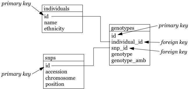
So how could we do that for the table above? Each row contains 3 different types of things: information about an individual (i.c. name and ethnicity), a SNP (i.c. the accession number, chromosome and position), and a genotype linking those two together (the genotype column, and the column containing the IUPAC ambiguity code for that genotype). To get to the second normal form, we need to put each of these in a separate table:
- The name of each table should be plural (not mandatory, but good practice).
- Each table should have a primary key, ideally named
id. Different tables can contain columns that have the same name; column names should be unique within a table, but can occur across tables. - The individual column is renamed to name, and snp to accession.
- In the genotypes table, individuals and SNPs are linked by referring to their primary keys (as used in the individuals and snps tables). Again best practice: if a foreign key refers to the id column in the individuals table, it should be named individual_id (note the singular).
- The foreign keys individual_id and snp_id in the genotypes table must be of the same type as the id columns in the individuals and snps tables, respectively.
The individuals table:
| id | name | ethnicity |
|---|---|---|
| 1 | individual_A | caucasian |
| 2 | individual_B | caucasian |
The snps table:
| id | accession | chromosome | position |
|---|---|---|---|
| 1 | rs12345 | 1 | 12345 |
| 2 | rs98765 | 1 | 98765 |
| 3 | rs28465 | 5 | 28465 |
The genotypes table:
| id | individual_id | snp_id | genotype | genotype_amb |
|---|---|---|---|---|
| 1 | 1 | 1 | A/A | A |
| 2 | 1 | 2 | A/G | R |
| 3 | 1 | 3 | G/T | K |
| 4 | 2 | 1 | A/C | M |
| 5 | 2 | 2 | G/G | G |
| 6 | 2 | 3 | G/G | G |
To generate these tables:
sqlite> DROP TABLE individuals;
sqlite> DROP TABLE snps;
sqlite> DROP TABLE genotypes;
sqlite> CREATE TABLE individuals (id INTEGER PRIMARY KEY, name STRING, ethnicity STRING);
sqlite> CREATE TABLE snps (id INTEGER PRIMARY KEY, accession STRING, chromosome STRING, position INTEGER);
sqlite> CREATE TABLE genotypes (id INTEGER PRIMARY KEY, individual_id INTEGER, snp_id INTEGER, genotype STRING, genotype_amb STRING);
sqlite> INSERT INTO individuals (name, ethnicity) VALUES ('individual_A','caucasian');
sqlite> INSERT INTO individuals (name, ethnicity) VALUES ('individual_B','caucasian');
sqlite> INSERT INTO snps (accession, chromosome, position) VALUES ('rs12345','1',12345);
sqlite> INSERT INTO snps (accession, chromosome, position) VALUES ('rs98765','1',98765);
sqlite> INSERT INTO snps (accession, chromosome, position) VALUES ('rs28465','5',28465);
sqlite> INSERT INTO genotypes (individual_id, snp_id, genotype, genotype_amb) VALUES (1,1,'A/A','A');
sqlite> INSERT INTO genotypes (individual_id, snp_id, genotype, genotype_amb) VALUES (1,2,'A/G','R');
sqlite> INSERT INTO genotypes (individual_id, snp_id, genotype, genotype_amb) VALUES (1,3,'G/T','K');
sqlite> INSERT INTO genotypes (individual_id, snp_id, genotype, genotype_amb) VALUES (2,1,'A/C','M');
sqlite> INSERT INTO genotypes (individual_id, snp_id, genotype, genotype_amb) VALUES (2,2,'G/G','G');
sqlite> INSERT INTO genotypes (individual_id, snp_id, genotype, genotype_amb) VALUES (2,3,'G/G','G');
Third normal form
In the third normal form, we try to eliminate unnecessary data from our database; data that could be calculated based on other things that are present. In our example table genotypes, the genotype and genotype_amb columns basically contain the same information, just using a different encoding. We could (should) therefore remove one of these. Our final individuals table would look like this:
| id | name | ethnicity |
|---|---|---|
| 1 | individual_A | caucasian |
| 2 | individual_B | caucasian |
The snps table:
| id | accession | chromosome | position |
|---|---|---|---|
| 1 | rs12345 | 1 | 12345 |
| 2 | rs98765 | 1 | 98765 |
| 3 | rs28465 | 5 | 28465 |
The genotypes table:
| id | individual_id | snp_id | genotype_amb |
|---|---|---|---|
| 1 | 1 | 1 | A |
| 2 | 1 | 2 | R |
| 3 | 1 | 3 | K |
| 4 | 2 | 1 | M |
| 5 | 2 | 2 | G |
| 6 | 2 | 3 | G |
To know what your database schema looks like, you can issue the .schema command in sqlite3. .tables gives you a list of the tables that are defined.
Other best practices
There are some additional guidelines that you can use in creating your database schema, although different people use different guidelines. What I do:
- No capitals in table or column names
- Every table name is plural (e.g.
genes) - The primary key of each table should be
id - Any foreign key should be the singular of the table name, plus “_id”. So for example, a genotypes table can have a sample_id column which refers to the id column of the samples table.
In some cases, I digress from the rule of “every table name is plural”, especially if a table is really meant to link to other tables together. A table genotypes which has an id, sample_id, snp_id, and genotype could e.g. also be called sample2snp.
SQL - Structured Query Language
Any interacting with data in RDBMS can happen through the Structured Query Language (SQL): create tables, insert data, search data, … There are two subparts of SQL:
DDL - Data Definition Language:
CREATE DATABASE test;
CREATE TABLE snps (id INT PRIMARY KEY AUTOINCREMENT, accession STRING, chromosome STRING, position INTEGER);
ALTER TABLE...
DROP TABLE snps;
For examples: see above.
DML - Data Manipulation Language:
SELECT
UPDATE
INSERT
DELETE
Some additional functions are:
DISTINCT
COUNT(*)
COUNT(DISTINCT column)
MAX(), MIN(), AVG()
GROUP BY
UNION, INTERSECT
We’ll look closer at getting data into a database and then querying it, using these four SQL commands.
Getting data in
INSERT INTO
There are several ways to load data into a database. The method used above is the most straightforward but inadequate if you have to load a large amount of data.
It’s basically:
sqlite> INSERT INTO <table_name> (<column_1>, <column_2>, <column_3>)
                               VALUES (<value_1>, <value_2>, <value_3>);
Importing a datafile
But this becomes an issue if you have to load 1,000s of records. Luckily, it’s possible to load data from a comma-separated file straight into a table. Suppose you want to load 3 more individuals, but don’t want to type the insert commands straight into the sql prompt. Create a file (e.g. called data.csv) that looks like this:
individual_C,african
individual_D,african
individual_C,asian
SQLite contains a .import command to load this type of data. Syntax: .import <file> <table>. So you could issue:
sqlite> .separator ','
sqlite> .import data.csv individuals
Aargh… We get an error!
Error: data.tsv line 1: expected 3 columns of data but found 2
This is because the table contains an ID column that is used as primary key and that increments automatically. Unfortunately, SQLite cannot work around this issue automatically. One option is to add the new IDs to the text file and import that new file. But we don’t want that, because it screws with some internal counters (SQLite keeps a counter whenever it autoincrements a column, but this counter is not adjusted if you hardwire the ID). A possible workaround is to create a temporary table (e.g. individuals_tmp) without the id column, import the data in that table, and then copy the data from that temporary table to the real individuals.
sqlite> .schema individuals
sqlite> CREATE TABLE individuals_tmp (name STRING, ethnicity STRING);
sqlite> .separator ','
sqlite> .import data.csv individuals_tmp
sqlite> INSERT INTO individuals (name, ethnicity) SELECT * FROM individuals_tmp;
sqlite> DROP TABLE individuals_tmp;
Your individuals table should now look like this (using SELECT * FROM individuals;):
| id | name | ethnicity |
|---|---|---|
| 1 | individual_A | caucasian |
| 2 | individual_B | caucasian |
| 3 | individual_C | african |
| 4 | individual_D | african |
| 5 | individual_E | asian |
Using scripting
There are different ways you can load data into an SQL database from scripting languages (I like to do this using Ruby, but as this is a Perl-oriented course we’ll look at that instead…) See Perl-DBI below where we devote a whole section to interfacing Perl to a database. In addition, you will see how to talk to an SQLite database from R in one of the following lectures.
Getting data out
Queries
Single tables
It is very simple to query a single table. The basic syntax is:
SELECT <column_name1, column_name2> FROM <table_name> WHERE <conditions>;If you want to see all columns, you can use “*” instead of a list of column names, and you can leave out the WHERE clause. The simplest query is therefore SELECT * FROM <table_name>;. So the <column_name1, column_name2> defines slices the table vertically while the WHERE clause slices it horizontally.
Data can be filtered using a WHERE clause. For example:
SELECT * FROM individuals WHERE ethnicity = 'african';
SELECT * FROM individuals WHERE ethnicity = 'african' OR ethnicity = 'caucasian';
SELECT * FROM individuals WHERE ethnicity IN ('african', 'caucasian');
SELECT * FROM individuals WHERE ethnicity != 'asian';
You often just want to see a small subset of data just to make sure that you’re looking at the right thing. In that case: add a LIMIT clause to the end of your query, which has the same effect as using head on the linux command-line. Please always do this if you don’t know what your table looks like because you don’t want to send millions of lines to your screen.
SELECT * FROM individuals LIMIT 5;
SELECT * FROM individuals WHERE ethnicity = 'caucasian' LIMIT 1;
If you just want know the number of records that would match your query, use COUNT(*):
SELECT COUNT(*) FROM individuals WHERE ethnicity = 'african';Using the GROUP BY clause you can aggregate data. For example:
SELECT ethnicity, COUNT(*) from individuals GROUP BY ethnicity;Combining tables
In the second normal form we separated several aspects of the data in different tables. Ultimately, we want to combine that information of course. This is where the primary and foreign keys come in. Suppose you want to list all different SNPs, with the alleles that have been found in the population:
SELECT snp_id, genotype_amb FROM genotypes;This isn’t very informative, because we get the uninformative numbers for SNPs instead of SNP accession numbers. To run a query across tables, we have to call both tables in the FROM clause:
SELECT snps.accession, genotypes.genotype_amb FROM snps, genotypes WHERE snps.id = genotypes.snp_id;What happens here?
- Both the snps and genotypes tables are referenced in the FROM clause.
- In the SELECT clause, we tell the query what columns to return. We prepend the column names with the table name, to know what column we actually mean (snps.id is a different column from individuals.id).
- In the WHERE clause, we actually provide the link between the 2 tables: the value for snp_id in the genotypes table should correspond with the id column in the snps table. What do you think would happen if we wouldn’t provide this WHERE clause? How many records would be returned?
Having to type the table names in front of the column names can become tiresome. We can however create aliases like this:
SELECT s.accession, g.genotype_amb FROM snps s, genotypes g WHERE s.id = g.snp_id;Now how do we get a list of individuals with their genotypes for all SNPs?:
SELECT i.name, s.accession, g.genotype_amb
FROM individuals i, snps s, genotypes g
WHERE i.id = g.individual_id
AND s.id = g.snp_id;
Output looks like this:
| name | accession | genotype_amb |
|---|---|---|
| individual_A | rs12345 | A |
| individual_A | rs98765 | R |
| individual_A | rs28465 | K |
| individual_B | rs12345 | M |
| individual_B | rs98765 | G |
| individual_B | rs28465 | G |
JOIN
Sometimes, though, we have to join tables in a different way. Suppose that our snps table contains SNPs that are nowhere mentioned in the genotypes table, but we still want to have them mentioned in our output:
sqlite> INSERT INTO snps (accession, chromosome, position) VALUES ('rs11223','2',11223);If we run the following query:
sqlite> SELECT s.accession, s.chromosome, s.position, g.genotype_amb
   ...> FROM snps s, genotypes g
   ...> WHERE s.id = g.snp_id
   ...> ORDER BY s.accession, g.genotype_amb;
We get the following output:
| chromosome | position | accession | genotype_amb |
|---|---|---|---|
| 1 | 12345 | rs12345 | A |
| 1 | 12345 | rs12345 | M |
| 1 | 98765 | rs98765 | G |
| 1 | 98765 | rs98765 | R |
| 5 | 28465 | rs28465 | G |
| 5 | 28465 | rs28465 | K |
But we actually want to have rs11223 in the list as well. Using this approach, we can’t because of the WHERE s.id = g.snp_id clause. The solution to this is to use an explicit join. To make things complicated, there are several types: inner and outer joins. In principle, an inner join gives the result of the intersect between two tables, while an outer join gives the results of the union. What we’ve been doing up to now is look at the intersection, so the approach we used above is equivalent to an inner join:
sqlite> SELECT s.accession, g.genotype_amb
   ...> FROM snps s INNER JOIN genotypes g ON s.id = g.snp_id
   ...> ORDER BY s.accession, g.genotype_amb;
gives:
| accession | genotype_amb |
|---|---|
| rs12345 | A |
| rs12345 | M |
| rs28465 | G |
| rs28465 | K |
| rs98765 | G |
| rs98765 | R |
A left outer join returns all records from the left table, and will include any matches from the right table:
sqlite> SELECT s.accession, g.genotype_amb
   ...> FROM snps s LEFT OUTER JOIN genotypes g ON s.id = g.snp_id
   ...> ORDER BY s.accession, g.genotype_amb;
gives:
| accession | genotype_amb |
|---|---|
| rs11223 | |
| rs12345 | A |
| rs12345 | M |
| rs28465 | G |
| rs28465 | K |
| rs98765 | G |
| rs98765 | R |
(Notice the extra line for rs11223!)
A full outer join, finally, return all rows from the left table, and all rows from the right table, matching any rows that should be.
Export to file
Often you will want to export the output you get from an SQL-query to a file (e.g. CSV) on your operating system so that you can use that data for external analysis in R or for visualization. This is easy to do. Suppose that we want to export the first 5 lines of the snps table into a file called 5_snps.csv. You do that like this:
sqlite> .header on
sqlite> .mode csv
sqlite> .once 5_snps.csv
sqlite> SELECT * FROM snps LIMIT 5;
If you now exit the sqlite prompt (with .quit), you should see a file in the directory where you were that is called 5_snps.csv.
Additional functions
NULL
What if you want to search for something that is not there? What if you want to search for the SNPs that are not in genes?
| snp-id | gene |
|---|---|
| rs1234 | gene_A |
| rs2345 | gene_A |
| rs3456 | gene_B |
| rs4567 | |
| rs6789 | gene_C |
| rs7890 | gene_C |
We cannot SELECT * FROM snps WHERE gene = ""; because that is searching for an empty string which is not the same as a missing value. To get to rs4567 you can issue SELECT * FROM snps WHERE gene IS NULL; or to get the rest SELECT * FROM snps WHERE GENE IS NOT NULL;. Note that it is IS NULL and not = NULL…
AND, OR, IN
Your queries might need to combine different conditions:
sqlite> SELECT * FROM snps WHERE chromosome = '1' AND position < 40000;
sqlite> SELECT * FROM snps WHERE chromosome = '1' OR chromosome = '5';
sqlite> SELECT * FROM snps WHERE chromosome IN ('1','5');
DISTINCT
Whenever you want the unique values in a column: use DISTINCT in the SELECT clause:
sqlite> SELECT genotype_amb FROM genotypes;
genotype_amb
A
R
K
M
G
G
sqlite> SELECT DISTINCT genotype_amb FROM genotypes;
genotype_amb
A
G
K
M
R
DISTINCT automatically sorts the results.
ORDER BY
sqlite> SELECT * FROM snps ORDER BY chromosome;
sqlite> SELECT * FROM snps ORDER BY accession DESC;
COUNT
For when you want to count things:
sqlite> SELECT COUNT(*) FROM genotypes WHERE genotype_amb = 'G';MAX(), MIN(), AVG()
…act as you would expect (only works with numbers, obviously):
sqlite> SELECT MAX(position) FROM snps;GROUP BY
GROUP BY can be very useful in that it first aggregates data. It is often used together with COUNT, MAX, MIN or AVG:
sqlite> SELECT genotype_amb, COUNT(*) FROM genotypes GROUP BY genotype_amb;
sqlite> SELECT genotype_amb, COUNT(*) AS c FROM genotypes GROUP BY genotype_amb ORDER BY c DESC;
sqlite> SELECT chromosome, MAX(position) FROM snps GROUP BY chromosome ORDER BY chromosome;| genotype_amb | c |
|---|---|
| G | 2 |
| A | 1 |
| K | 1 |
| M | 1 |
| R | 1 |
| chromosome | MAX(position) |
|---|---|
| 1 | 98765 |
| 2 | 11223 |
| 5 | 28465 |
UNION, INTERSECT
It is sometimes hard to get the exact rows back that you need using the WHERE clause. In such cases, it might be possible to construct the output based on taking the union or intersection of two or more different queries:
sqlite> SELECT * FROM snps WHERE chromosome = '1';
sqlite> SELECT * FROM snps WHERE position < 40000;
sqlite> SELECT * FROM snps WHERE chromosome = '1' INTERSECT SELECT * FROM snps WHERE position < 40000;| id | accession | chromosome | position |
|---|---|---|---|
| 1 | rs12345 | 1 | 12345 |
LIKE
Sometimes you want to make fuzzy matches. What if you’re not sure if the ethnicity has a capital or not?
sqlite> SELECT * FROM individuals WHERE ethnicity = 'African';returns no results…
sqlite> SELECT * FROM individuals WHERE ethnicity LIKE '%frican';LIMIT
If you only want to get the first 10 results back (e.g. to find out if your complicated query does what it should do without running the whole actual query), use LIMIT:
sqlite> SELECT * FROM snps LIMIT 2;Subqueries
As we mentioned in the beginning, the general setup of a SELECT is:
SELECT <column_names>
FROM <table>
WHERE <condition>;
But as you’ve seen in the examples above, the output from any SQL query is itself basically a table. So we can actually use that output table to run another SELECT. For example:
sqlite> SELECT *
   ...> FROM (
   ...>        SELECT *
   ...>        FROM snps
   ...>        WHERE chromosome IN ('1','5'))
   ...> WHERE position < 40000;
Of course, you can use UNION and INTERSECT in the subquery as well…
Another example:
sqlite> SELECT COUNT(*)
   ...> FROM (
   ...>        SELECT DISTINCT genotype_amb
   ...>        FROM genotypes);
Public bioinformatics databases
Sqlite is a light-weight system for running relational databases. If you want to make your data available to other people it’s often better to use systems such as MySQL. The data behind the Ensembl genome browser, for example, is stored in a relational database and directly accessible through SQL as well.
To access the last release of human from Ensembl: mysql -h ensembldb.ensembl.org -P 5306 -u anonymous homo_sapiens_core_70_37. To get an overview of the tables that we can query: show tables.
To access the hg19 release of the UCSC database (which is also a MySQL database): mysql --user=genome --host=genome-mysql.cse.ucsc.edu hg19.
Views
By decomposing data into different tables as we described above (and using the different normal forms), we can significantly improve maintainability of our database and make sure that it does not contain inconsistencies. But at the other hand, this means it’s a lot of hassle to look at the actual data: to know what the genotype is for SNP rs12345 in individual_A we cannot just look it up in a single table, but have to write a complicated query which joins 3 tables together. The query would look like this:
SELECT i.name, i.ethnicity, s.accession, s.chromosome, s.position, g.genotype_amb
FROM individuals i, snps s, genotypes g
WHERE i.id = g.individual_id
AND s.id = g.snp_id;
Output looks like this:
| name | ethnicity | accession | chromosome | position | genotype_amb |
|---|---|---|---|---|---|
| individual_A | caucasian | rs12345 | 1 | 12345 | A |
| individual_A | caucasian | rs98765 | 1 | 98765 | R |
| individual_A | caucasian | rs28465 | 5 | 28465 | K |
| individual_B | caucasian | rs12345 | 1 | 12345 | M |
| individual_B | caucasian | rs98765 | 1 | 98765 | G |
| individual_B | caucasian | rs28465 | 5 | 28465 | G |
There is however a way to make this easier: you can create views on the data. This basically saves the whole query and gives it a name. You do this by adding CREATE VIEW some_name AS to the front of the query, like this:
CREATE VIEW v_genotypes AS
SELECT i.name, i.ethnicity, s.accession, s.chromosome, s.position, g.genotype_amb
FROM individuals i, snps s, genotypes g
WHERE i.id = g.individual_id
AND s.id = g.snp_id;
You can think of this as if you had made a new table with the name v_genotypes that you can use just like any other table, for example:
SELECT *
FROM v_genotypes g
WHERE g.genotype_amb = 'R';
The difference with an actual table is, however, that the result of the view is actually not stored itself. Whenever you do SELECT * FROM v_genotypes, it will actually perform the whole query in the background.
Note: to make sure that I can tell by the name if something is a table or a view, I always add a v_ in front of the name that I give to the view.
Pivot tables
In some cases, you want to violate the 1st normal form, and have different columns represent the same type of data. A typical example is when you want to analyze your data in R using a dataframe. Let’s say we have expression values for different genes in different individuals. Being good programmers, we saved this data in the database like this:
| individual | gene | expression |
|---|---|---|
| individual_A | gene_A | 2819 |
| individual_A | gene_B | 1028 |
| individual_A | gene_C | 3827 |
| individual_B | gene_A | 1928 |
| individual_B | gene_B | 999 |
| individual_B | gene_C | 1992 |
In R, you will however probably want a dataframe that looks like this:
| gene | individual_A | individual_B |
|---|---|---|
| gene_A | 2819 | 1928 |
| gene_B | 1028 | 999 |
| gene_C | 3827 | 1992 |
This is called a pivot table, and there are several ways to create these in SQLite. The method presented here is taken from http://bduggan.github.io/virtual-pivot-tables-opensqlcamp2009-talk/. To create such table (and store it in a view), you have to use group_concat and group_by:
CREATE VIEW v_pivot_expressions AS
SELECT gene,
       GROUP_CONCAT(CASE WHEN individual = 'individual_A' THEN expression ELSE NULL END) AS individual_A,
       GROUP_CONCAT(CASE WHEN individual = 'individual_B' THEN expression ELSE NULL END) AS individual_B
FROM expressions
GROUP BY gene;
Drawbacks of relational databases
Relational databases are great. They can be a big help in storing and organizing your data. But they are not the ideal solution in all situations.
Scalability
Relational databases are only scalable in a limited way. The fact that you try to normalize your data means that your data is distributed over different tables. Any query on that data often requires extensive joins. This is OK, until you have tables with millions of rows. A join can in that case a very long time to run.
[Although outside of the scope of this lecture.] One solution sometimes used is to go for a star-schema rather than a fully normalized schema. Or using a NoSQL database management system that is horizontally scalable (document-oriented, column-oriented or graph databases).
Modeling
Some types of information are difficult to model when using a relational paradigm. In a relational database, different records can be linked across tables using foreign keys. If you’re however really interested in the relations themselved (e.g. social graphs, protein-protein-interaction, …) you are much better of to use a real graph database (e.g. neo4j) instead of a relational database. In a graph database finding all neighbours-of-neighbours in a graph of 50 members (basically) takes as long as in a graph with 50 million members.
Drawback exercise
Suppose you want to model a social graph. People have names, and know other people. Every “know” is reciprocal (so if I know you then you know me). The data might look like this:
Tim knows Terry
Tom knows Terry
Terry knows Gerry
Gerry knows Rik
Gerry knows James
James knows John
Fred knows James
Frits knows Fred
In table format:
| knower | knowee |
|---|---|
| Tim | Terry |
| Tom | Terry |
| Terry | Gerry |
| Gerry | Rik |
| Gerry | James |
| James | John |
| Fred | James |
| Frits | Fred |
Given that you really want to have this in a relational database, how would you find out who are the friends of the friends of James?