In this exercise, we will use the Processing tool (http://processing.org) to generate visualizations based on a flights dataset. In particular, we will use the python mode (http://py.processing.org). This tutorial holds numerous code snippets that can by copy/pasted and modified for your own purpose. The contents of this tutorial is available under the CC-BY license.

The tutorial is written in a very incremental way. We start with something simple, and gradually add little bits and pieces that allow us to make more complex visualizations. So make sure to not skip parts of the tutorial: everything depends on everything that precedes it.

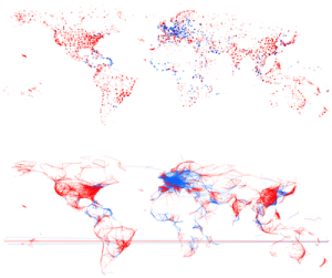
Figure 1 - A pretty picture

Introduction to Processing

py.processing is a language based on python, with its own development environment.

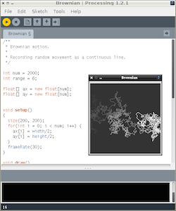
Figure 2 - The Processing IDE

Download and install py-processing

Processing can be downloaded from http://processing.org/download/.

• For Windows: Double-click the zip-file; there should be a processing.exe file which is your program.
• For Mac: Just double-click the downloaded file.
• For linux: Download the .tgz file, and run tar -xvzf that_file.tgz.

To install python mode, click on the button in the top-right corner, select “Add Mode…” from the drop-down box, and choose “Python”. Then re-start Processing.

A minimal script

A minimal script is provided below.

Script 1

size(400,400)

fill(255,0,0)
ellipse(100,150,20,20)

fill(0,255,0)
rect(200,200,50,60)

stroke(0,0,255)
strokeWeight(5)
line(150,5,150,50)

This code generates the following image:

Figure 3 - Minimal output

The numbers at the front of each line are the line numbers and are actually not part of the program. We’ve added them here to be able to refer to specific lines. So if you type in this piece of code, do not type the line numbers.

Let’s walk through each line. The script is made up of a list of statements. The first line in the script size(400,400) sets the dimensions of the resulting image. In this case, we’ll generate a picture of 400x400 pixels. Next, (line 3) we set the colour of anything we draw to red. The fill function takes 3 parameters, which are the values for red, green, and blue (RGB), ranging from 0 to 255. We then draw an ellipse with its center at horizontal position 100 pixels and vertical position 150 pixels. Note that the vertical position counts from the top down instead of from the bottom up. The point (0,0) is at the top left rather than the bottom left… For the ellipse we set both the horizontal and vertical diameter to 20 pixels, which results in a circle. The next thing we do (line 6) is set the colour of anything that we will draw to green fill(0,255,0), and draw a rectangle at position (200,200) with width set to 50 and height to 60.

Finally, we set the colour of lines to blue (stroke(0,0,255)), the stroke weight to 5 pixels strokeWeight(5), and draw a line line(150,5,150,50). This line runs from point (150,5) to (150,50).

Both fill and stroke are used to set colour: fill to set the colour of the shape, stroke to set the colour of the border around that shape. In case of lines, only the stroke colour can be set.

Several drawing primitives exist, including line, rect, triangle, and ellipse (a circle is an ellipse with the same horizontal and vertical radius). A treasure trove of information for these is available in the Python Processing reference pages.

Apart from these primitives, Processing contains functions that modify properties of these primitives. These include setting the fill color (fill), color of lines (stroke), and line weight (lineWeight). Again, the reference pages host all information.

Variables, loops and conditionals

What if we want to do something multiple times? Suppose we want to draw 10 lines underneath each other. We could do that like this:

Script 2

size(500,150)
background(255,255,255)
line(100,0,400,0)
line(100,10,400,10)
line(100,20,400,20)
line(100,30,400,30)
line(100,40,400,40)
line(100,50,400,50)
line(100,60,400,60)
line(100,70,400,70)
line(100,80,400,80)
line(100,90,400,90)

This generates this image:

Figure 4 - Parallel lines

Of course this is not ideal: what if we have 5,000 datapoints to plot? To handle real data, we will need variables, loops, and conditionals.

In the code block above, we can replace the hard-coded numbers with variables. These can be integers, floats, strings, arrays, etc. startX = 100 creates a new variable called startX and gives it the value of 100.

Script 3

size(500,150)
startX = 100
stopX = 400
background(255,255,255);
for i in range(0,9):
  line(startX,i*10,stopX,i*10)

We first set the variables startX and stopX to 100 and 400. We then loop over values i, which start at 0 and go up to 9. In each loop, a line is drawn.

Whitespace is very important in python: it defines code blocks. In the for-loop above, line 6 is indented relative to line 5. This means that line 6 is part of the block started at line 5. In other languages (java, C, perl, ruby, …), you will for example see curly brackets ({}) used instead of whitespace to define blocks. A for-loop in java for example can look like this:

for ( int i = 0; i < 10; i++ ) { println "Variable i is not " + i };

As you can see, in java curly brackets have the same role as whitespace in python. This also means that the following code would not work, and will give an IndentationError:

for i in range(0,9):
  print i

We can use conditionals to for example distinguish odd or even lines by colour.

Script 4

size(500,150)
startX = 100
stopX = 400
background(255,255,255)
strokeWeight(2)
for i in range(0,9):
  if i%2 == 0:
    stroke(255,0,0)
  else:
    stroke(0,0,255)
    line(startX, i*10, stopX, i*10)

In this code snippet, we check in each loop if i is even or odd, and let the stroke colour depend on that result. An if-clause has the following form:

if *condition*:
    # do something
else:
    # do something else

The condition i%2 == 0 means: does dividing the number i with 2 result in a remainder of zero? Note that we have to use 2 equal-signs here (==) instead of just one (=). This is so to distinguish between a test for equality, and an assignment. Don’t make errors against this…

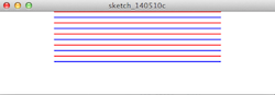
Figure 5 - Odd and even lines

Exercise data

The data for this exercise concerns flight information between different cities. Each entry in the dataset contains the following fields:

• from_airport
• from_city
• from_country
• from_long
• from_lat
• to_airport
• to_city
• to_country
• to_long
• to_lat
• airline
• airline_country
• distance

Getting the data

First, download this csv file somewhere on your computer. There are 3 ways to get the data into Processing: 1. First save your sketch. In the directory where you saved it, create a new folder called data. Copy the downloaded file into this data directory. 1. Or: drag the file onto your Processing IDE. 1. Or: Go to Sketch => Add file...

Accessing the data from Processing

Let’s write a small script in Processing to visualize this data. The visual encoding that we’ll use for each flight will be the following:

• x position is defined by longitude of departure airport
• y position is defined by latitude of departure airport

Script 5

table = loadTable("flights.csv","header")

size(800,400)
noStroke()
fill(0,0,255,10)

background(255,255,255)
for row in table.rows():
  from_long = row.getFloat("from_long")
  from_lat = row.getFloat("from_lat")
  x = map(from_long,-180,180,0,width)
  y = map(from_lat,-90,90,height,0)
  ellipse(x,y,3,3)

The resulting image:

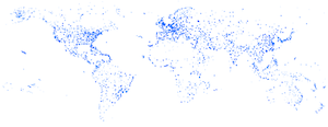
Figure 6 - Departure airports

You can see that the resulting image shows a map of the world, with areas with high airport density clearly visible. Notice that the data itself does not contain any information where the continents, oceans and coasts are; still, these are clearly visible in the image.

Let’s go through the code:

• Line 1 - The data from the file “flights.csv” is read into a variable table. The "header" indicates that the first line of the file is a list of column headers.
• Line 4 - noStroke() tell Processing to not draw the border around disks, rectangles or other elements.
• Line 8 - This is another way to loop over a collection, instead of the for i in range(0,9): we used before. In this line, we loop over all table.rows(), and each time we put the new row into a variable row.
• Line 9 - row.getFloat("from_long") extracts the value from the from_long column from that row and makes it a float. This is then stored in the variable from_long.
• Line 11 - In this line, we transform the longitude value to a value between 0 and the width of our canvas.

The map function is very useful. It is used to rescale values. In our case, longitude values range from -180 to 180. The x position of the dots on the screen, however, have to be between 0 and 800 (because that’s the width of our canvas, as set in canvase(800,800);). In this case, we can even use the variable width instead of 800, because width and height are set automatically when we call the statement size(800,800);. You see that the map function for y recalculates the from_lat value to something between height and 0, instead of between 0 and height. The reason is that the origin of our canvas is at the top-left corner instead of the bottom-left one so we have to flip coordinates.

We can add additional information to this visualization. In the next code block, we alter our script so that colour of the dots is red for domestic flights and blue for international flights. In addition, the size of the dots is proportional to the distance of that particular flight.

Script 6

table = loadTable("flights.csv","header")

size(800,400)
noStroke()
fill(0,0,255,10)

background(255,255,255)
for row in table.rows():
  from_long = row.getFloat("from_long")
  from_lat = row.getFloat("from_lat")
  from_country = row.getString("from_country")
  to_country = row.getString("to_country")
  distance = row.getInt("distance")

  x = map(from_long,-180,180,0,width)
  y = map(from_lat,-90,90,height,0)
  if from_country == to_country:
    fill(255,0,0,10)
  else:
    fill(0,0,255,10)
  r = map(distance,1,15406,3,15)

  ellipse(x,y,r,r)

In line 21, we rescale the value of the distance (min = 1, max = 15406) to a minimum of 3 and maximum of 15. That value is than used as the radius r.

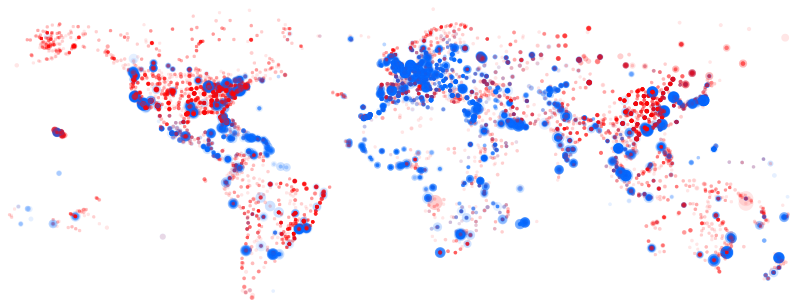
Figure 7 - Domestic vs international flights

From this picture, we can deduce many things:

• Airports tend to be located on land => plotting latitude and longitude recreates a worldmap.
• Blue international flights tend to depart from coastal regions.
• There are few domestic flights within Europe.
• Longer flights (departure airports with larger radius) tend to leave in coastal regions

Interactivity and defining functions

It is often the interactivity in data visualization that helps gaining insights in that data and finding new hypotheses. Up until now, we have generated static images. How can we add interactivity?

As a first use case, say that we want the radius of the dots to depend on the position of the mouse instead of the distance of the flight: if our mouse is at the left of the image, all dots should be small; if it is at the right, they should be large. We will change the line float r = map(distance,1,15406,3,15); to include information on the mouse position.

This time, instead of creating a simple image, this image will have to be redrawn constantly taking into account the mouse position. For this, we have to rearrange our code a little bit. Some of the code has to run only once to initialize the visualization, while the rest of the code has to be rerun constantly. We do this by putting the code that we have either in the setup() or the draw() function:

## define global variables here
def setup():
  # code that has to be run only once
def draw():
  # code that has to be rerun constantly`

A function definition (such as setup and draw) in python always has the same elements:

1. The def keyword (for “define”)
2. The name of the function
3. The names of parameters, between parentheses
4. The actual code of the function, as an indented code block

Both the setup() and the draw() functions don’t take any parameters, so we just use empty parentheses.

The setup() function is only run once; the draw() function is run by default 60 times per second.

Let’s put all statements we had before into one of these two functions:

Script 7

def setup():
  global table
  table = loadTable("flights.csv","header")
  size(800,400)
  noStroke()

def draw():
  global table
  background(255,255,255)
  for row in table.rows():
    from_long = row.getFloat("from_long")
    from_lat = row.getFloat("from_lat")
    from_country = row.getString("from_country")
    to_country = row.getString("to_country")
    distance = row.getInt("distance")

    x = map(from_long,-180,180,0,width)
    y = map(from_lat,-90,90,height,0)
    if from_country == to_country:
      fill(255,0,0,10)
    else:
      fill(0,0,255,10)
    r = map(distance,1,15406,3,15)

    ellipse(x,y,r,r)

The draw() function is run 60 times per second. This means that 60 times per second each line in the input table is processed again to draw a new circle. As this is quite compute intensive, your computer might actually not be able to redraw 60 times per second, and show some lagging. For simplicity’s sake, we will however not go into optimization here.

Some things to note:

• We have to define the table variable and load the actual data (using loadTable) at the top.
• We have to set the background every single redraw. If we wouldn’t, each picture is drawn on top of the previous one.

Now how do we adapt this so that the radius of the circles depends on the x-position of my pointer? Luckily, Processing provides two variables called mouseX and mouseY that are very useful. mouseX returns the x position of the pointer. So basically the only thing we have to do is replace float r = map(distance, 0, 15406, 3, 15); with float r = map(mouseX, 0, 800, 3, 15); (Note that we changed the 15406 to 800.) If we do that, and our mouse is towards the right side of the image, we get the following picture:

Figure 8 - Large dots

Some optimization Let’s optimize this code a tiny bit. We could for example remove the lines that handle the distance because we don’t use them. However, we’ll leave those in because we’ll use them in the next example… Something else that we can do is limit the number of times the picture is redrawn. As long as I don’t move my mouse I don’t have to redraw the picture. To do that, we add noLoop(); to the setup() function, and add a new function at the bottom, called mouseMoved(). In this new function, we tell Processing to redraw() the canvas. The resulting code looks like this:

Script 8

def setup():
  global table
  table = loadTable("flights.csv","header")
  size(800,400)
  noStroke()
  noLoop()

def draw():
  background(255,255,255)
  for row in table.rows():
    from_long = row.getFloat("from_long")
    from_lat = row.getFloat("from_lat")
    from_country = row.getString("from_country")
    to_country = row.getString("to_country")
    distance = row.getInt("distance")

    x = map(from_long,-180,180,0,width)
    y = map(from_lat,-90,90,height,0)
    if from_country == to_country:
      fill(255,0,0,10)
    else:
      fill(0,0,255,10)
    r = map(mouseX,0,800,3,15)

    ellipse(x,y,r,r)

def mouseMoved():
  redraw()

More useful interactivity

This interactivity can be made more useful: we can use the mouse pointer as a filter. For example: if our mouse is at the left only short distance flights are drawn; if our mouse is at the right only long distance flights are drawn.

Script 9

def setup():
  global table
  table = loadTable("flights.csv","header")    
  size(800,400)
  noStroke()
  noLoop()

def draw():
  background(255,255,255)
  for row in table.rows():
    distance = row.getInt("distance")
    mouseXMin = mouseX - 25
    mouseXMax = mouseX + 25
    minDistance = map(mouseXMin,0,800,0,15406)
    maxDistance = map(mouseXMax,0,800,0,15406)

    if minDistance < distance and distance < maxDistance:
      from_long = row.getFloat("from_long")
      from_lat = row.getFloat("from_lat")
      from_country = row.getString("from_country")
      to_country = row.getString("to_country")

      x = map(from_long,-180,180,0,width)
      y = map(from_lat,-90,90,height,0)
      if from_country == to_country:
        fill(255,0,0,10)
      else:
        fill(0,0,255,10)

      ellipse(x,y,3,3)

def mouseMoved():
  redraw()

We will only draw flights if their duration is between a calculated minDistance and maxDistance. That’s what we do on line 17. Of course we first have to calculate minDistance and maxDistance. That’s what we do on lines 12 to 15. In lines 12 and 13, we say that we will be looking 25 pixels at either side of the mouse position. If the pointer is at position 175, mouseMin is set to 150 and mouseMax to 200. This pixelrange is then translated into distance range on lines 14 and 15.

Now it gets interesting. We can now look a bit deeper into the data… If we have our mouse at the left side of the image, it looks like this:

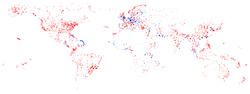
Figure 9 - Short distance flights

Having the mouse in the middle to the canvas gives us this image:

Figure 10 - Medium distance flights

Playing with this visualization, there are some signals that pop up. Moving left and right at about 70-90 pixels from the left, we see a “snake” moving along the north-east coast of Brazil (see Figure below, also indicating position of mouse). This indicates that most of these flights probably go to the same major city in that country. Other dynamic patterns appear in Europe as well. In Figure 10, some dots appear to be darker than others. Why do you think this is?

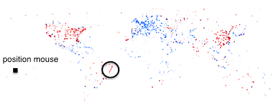
Figure 11 - A snake in Brazil

Buttons and sliders

Of course many tools have buttons and sliders. Let’s implement those in Processing. Instead of using the mouse position as a filter as before, why don’t we make a slider to do the same? Unfortunately, this is a bit more complex than it should be… So let’s first start with a button. To create a button, what we basically do is draw a rectangle, and check if the mouse position is within the area of that rectangle when we press the mouse button.

Script 10

def setup():
  global table
  table = loadTable("flights.csv","header")
  size(800,400)
  noStroke()
  noLoop()
  global grey
  grey = True

def draw():
  global grey
  background(255,255,255)
  fill(100,100,100)
  rect(50,100,20,20)
  for row in table.rows():
    distance = row.getInt("distance")
    mouseXMin = mouseX - 25
    mouseXMax = mouseX + 25
    minDistance = map(mouseXMin, 0, 800, 0, 15406)
    maxDistance = map(mouseXMax, 0, 800, 0, 15406)

    if minDistance < distance and distance < maxDistance:
      from_long = row.getFloat("from_long")
      from_lat = row.getFloat("from_lat")
      from_country = row.getString("from_country")
      to_country = row.getString("to_country")

      x = map(from_long,-180,180,0,width)
      y = map(from_lat,-90,90,height,0)

      if grey == True:
        fill(100,100,100,10)
      else:
        if from_country == to_country:
          fill(255,0,0,10)
        else:
          fill(0,0,255,10)

      ellipse(x,y,3,3)

def mouseClicked():
  global grey

  if mouseX > 50 and mouseX < 70 and mouseY > 100 and mouseY < 120:
    print('before :' + str(grey))
    if grey == True:
      grey = False
    else:
      grey = True
    print('after :' + str(grey))
  redraw()

def mouseMoved():
  redraw()

Now, we basically keep track of a variable called grey which can be true or false (such variable is called a “boolean”). If it is true then all points will be drawn in grey; if it is false then the points will be blue or red just like before.

The variable grey should be a “global” variable which is visible to the setup(), draw(), and mouseClicked() methods. To do this, we add global grey to each of these methods to indicate that they should not create their own grey variable, but use a global one.

We give the variable grey the value of true in the setup (line 7-8). Then, we draw a little square (line 13-14) just so that we have something to point at. Next, we change the line 25-28 from script 9 into line 31-37 in script 10. This first checks if the boolean grey is set to true, and sets the fill colour based on that information. Finally, we create a new method called mouseClicked (line 41-51) to handle the actual click event itself. This method (which really must be called “mouseClicked”) will be run every time you click the mouse. If you do so, it will check if the position of the mouse is within the range of the rectangle that we drew in the beginning. If it is, it changes the value of grey and redraws the map. See the reference guide on the Processing.org website for more information on mouseClicked().

Note that there is basically no connection between the rectangle we draw at line 14 and the actual click event: we have to check if our mouse is over the rectangle ourselves; we’re not able to say “if this rectangle is clicked”. We could just as well remove line 14 (so that we don’t see a rectangle) and the visualization would still work exactly the same. The only problem would be that you wouldn’t know where the region that we define in lines 44 actually is…

Now let’s implement an actual slider. This looks a lot like what we had before in script 9, but we obviously have to change some things. Let’s start with the final script, which was adapted from script 9:

Script 11

def setup():
  global table
  global circlePosition
  table = loadTable("flights.csv","header")
  size(800,400)
  noLoop()
  circlePosition = 50

def draw():
  global circlePosition
  background(255,255,255)
  stroke(150,150,150)
  line(50,150,150,150) # draw the line of 100 pixels long
  noStroke()
  fill(150,150,150)
  ellipse(circlePosition,150,10,10)

  circleXMin = circlePosition - 2
  circleXMax = circlePosition + 2
  minDistance = map(circleXMin, 50, 150, 0, 15406)
  maxDistance = map(circleXMax, 50, 150, 0, 15406)

  for row in table.rows():
    distance = row.getInt("distance")

    if minDistance < distance and distance < maxDistance:
      from_long = row.getFloat("from_long")
      from_lat = row.getFloat("from_lat")
      from_country = row.getString("from_country")
      to_country = row.getString("to_country")

      x = map(from_long,-180,180,0,width)
      y = map(from_lat,-90,90,height,0)

      if from_country == to_country:
        fill(255,0,0,10)
      else:
        fill(0,0,255,10)
      ellipse(x,y,3,3)

def mouseDragged():
  global circlePosition
  if abs(mouseX - circlePosition) <= 5 and abs(mouseY - 150) <= 5 and mouseX >= 50 and mouseX <= 150:
    circlePosition = mouseX
    redraw()

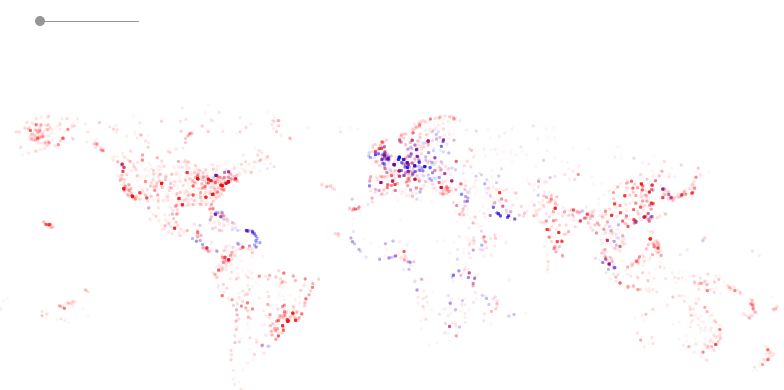
Figure 12 - A slider

So what changed? We now define a variable called circlePosition in the setup(), draw() and mouseDragged() methods, and give it an initial value of 50 (line 7). At the start of the draw() function (lines 12 to 16), we also draw a line that will serve as a guide as well as the actual circle. Furthermore, we change lines (lines 18 to 21) to refer to the circlePosition instead of mouseX. Note that that includes using +/- 2 instead of +/- 25 as a buffer, and using the minimum and maximum values of the line (i.e. 50 and 150) instead of those of the mouse in the map functions. Finally, we write the mouseDragged() function at the bottom (lines 41 to 45). A “mouse-drag” in Processing-speak means: pressing the mouse button, then moving the mouse to another position, and finally releasing the mouse button. The mouseDragged() function looks a lot like the mouseClicked() function in script 10. We want to make sure that we are on top of the circle when we start dragging (both horizontally and vertically; line 43). Also, we need to make sure that we cannot drag the circle further than the minimum or maximum value. If the situation complies to these three conditions, we change the circlePosition to mouseX, which basically means that the circle follows the mouse. Don’t forget the redraw() or the scene will not be updated. Question: what happens if you drag the mouse too fast? Why is that? And just for laughs: remove the and mouseX >= 50 and mouseX <= 150, and see what happens if you start interacting with the visualization…

Brushing and linking

Very often, you will want to create views that show different aspects of the same data. In our flights case, we might want to have both a map and a histogram of the flight distances. To be able to do this, we will have to look at how to create objects.

Working with objects

Dogs

The code that we have been writing so far is what they call “imperative”: the code does not know what we are talking about (i.e. flight data); it just performs a single action for each line in the file. As a result, all things (dots) on the screen are completely independent. They do not know of each other’s existence. To create linked views, however, we will need to make these visuals more self-aware, which we do by working with objects. Objects are members of a specific class. For example, Rusty, Duke and Lucy are three dogs; in object-oriented speak, we say that Rusty, Duke and Lucy are “objects” of the “class” dog. Of course, all dogs have types of properties in common: they have names, have a breed, a weight, etc. At the same time, they share some methods, for example: they can all bark, eat, pee, …

In object-oriented programming, we first define classes that completely describe the properties and methods of that type of object. Have a look at this bit of code that defines and creates a dog.

Script 12

class Dog:  
  def __init__(self, n, b, w):
    self.name = n
    self.breed = b
    self.weight = w

  def bark(self):
    print("My name is " + self.name + ", I'm a " + self.breed + ", and I weigh " + str(self.weight) + " kg")

  def eat(self):
    print("I am " + self.name + " and I ate")

  def pee(self):
    print("I am " + self.name + " and I've got wet legs now")    

def setup():
  size(800,800)

  dog1 = Dog("Buddy","Rottweiler",19)
  dog2 = Dog("Lucy","Terrier",8)

  dog1.bark()
  dog1.eat()
  dog1.pee()
  dog2.bark()
  dog2.eat()
  dog2.pee()

When you run this code, you will see an empty picture (because we didn’t draw anything), but you will also see some text appear in the black terminal underneath your code. That text should be:

My name is Buddy, I'm a Rottweiler, and I weight 19.0 kg
I am Buddy and I ate
I am Buddy and I've got wet legs now
My name is Lucy, I'm a Terrier, and I weight 8.0 kg
I am Lucy and I ate
I am Lucy and I've got wet legs now

So what did we do? Outside of the setup() method, in lines 1 to 14, we defined a new class, called Dog (notice the uppercase “D”). In such class, we want to do 2 things: (1) define a method to create a new member of this class (lines 2 to 5), and (2) define any additional methods of the class (lines 7 to 14).

The method to create a new object of the class is called __init__() (note the 2 underscores on either side). Also, you see here that every method should have self as the first argument. This argument is hidden in the calling code, though. For example, you see that the creation of a new object takes 4 parameters (line 2), but when we actually call that function to create dog1 (line 19), we only provide 3. The self is automatic. The other parameters (the things between parentheses) can be assigned to properties of the objects.

In our little example here, the methods bark(), eat() and pee() don’t do anything else than sending some text to the console, using print().

Now what does this actually mean? We can create new objects just like we create variables before, for example the startX = 100 in script 4. Just like we did in the previous scripts, we create 2 new variables (of the type Dog).

dog1 = Dog("Buddy","Rottweiler",19)

Once we have these objects, we can call the methods on them that we defined in the class definition, as is shown in lines 22 to 27.

One flight

So what could a flight class look like? Let’s alter this code so that we use a Flight class.

Script 13

class Flight:  
  def __init__(self, d,flo,fla,tlo,tla,fc,tc):
    self.distance = d
    self.from_long = flo
    self.from_lat = fla
    self.to_long = tlo
    self.to_lat = tla
    self.from_country = fc
    self.to_country = tc

    self.x = map(self.from_long, -180,180,0,width)
    self.y = map(self.from_lat, -180,180,height,0)

  def drawDepartureAirport(self):
    ellipse(self.x, self.y, 3,3)


def setup():
  global my_flight
  size(800,800)
  fill(0,0,255,10)
  my_flight = Flight(1458, 61.838, 55.509, 38.51, 55.681, "Belgium", "Germany")

def draw():
  global my_flight
  background(255,255,255)
  my_flight.drawDepartureAirport()

For simplicity’s sake, we only draw a single flight in this example. So what did we do? We define the Flight class in lines 1 to 15. First, we create an __init__() method for creating new objects and assigning properties (line 2 to 12). We also include x and y here. These are the x- and y-positions on the screen as we used before. Even though these are computed, they are specific for a flight and we can therefore calculate them in the creation method and look at them as any other property of a flight.

In the setup() method, we create a new object/variable of the class Flight, that we give the name my_flight. Next, in the draw() method, we actually draw the flight (line 26). Notice here that we don’t write ellipse() or anything drawing-specific here. We write my_flight.draw() because any flight object knows how to draw itself. The drawDepartureAiport() method definition on lines 14 and 15 returns an ellipse whenever that method is called.

Many flights

In the code of script 13, we only drew one flight. Here is the same code as in script 13, but showing all flights.

Script 14

class Flight:  
  def __init__(self, d,flo,fla,tlo,tla,fc,tc):
    self.distance = d
    self.from_long = flo
    self.from_lat = fla
    self.to_long = tlo
    self.to_lat = tla
    self.from_country = fc
    self.to_country = tc

    self.x = map(self.from_long, -180,180,0,width)
    self.y = map(self.from_lat, -180,180,height,0)

  def drawDepartureAirport(self):
    ellipse(self.x, self.y, 3,3)

def setup():
  global flights
  flights = []
  size(800,800)
  noStroke()
  noLoop()
  fill(0,0,255,10)
  table = loadTable("flights.csv","header")
  for row in table.rows():
    distance = row.getInt("distance")
    from_long = row.getFloat("from_long")
    from_lat = row.getFloat("from_lat")
    to_long = row.getFloat("to_long")
    to_lat = row.getFloat("to_lat")
    from_country = row.getString("from_country")
    to_country = row.getString("to_country")
    this_flight = Flight(distance,from_long,from_lat,to_long,to_lat,from_country,to_country) flights.append(this_flight)

def draw():
  global flights
  background(255,255,255)
  for flight in flights:
    flight.drawDepartureAirport()

As always, let’s see what is different in this script relative to the previous one. For starters, the Flight class is exactly the same as in script 13. Some parts are the same as in script 11, before we started working with these object things. But these are the really new things:

• On line 18 and 19, we define a global variable flights and make it an empty array.
• On line 25 to 34, we go over each line in the file, get the required columns for that row, and create a new flight object. We then add (append) that new flight to the flights array (line 34).
• In the draw() method, we also define that same global flights.
• On lines 40 and 41, we loop over all flights and let each draw itself.

The resulting picture should be the same as that from script 5 (i.e. Figure 6).

Linking two copies of the departure plots

Now that we work with objects, we can start implementing brushing and linking. Let’s first look at the brushing.

Brushing

Let’s change the code from script 14 a bit, so that all objects that are in the vicinity (e.g. within 10 pixels) of the mouse position are “active”. To do this, we’ll (1) add a new function to the Flight class, which checks if an object (i.e. flight) is selected/activated or not, and (2) change the drawDepartureAiport() function a bit to distinguish between selected and non-selected objects.

Add the following function to the Flight class:

def selected():
  if dist(mouseX, mouseY, self.x, self.y) < 10:
    return True
  else:
    return False

And change the drawDepartureAiport() function to this:

def drawDepartureAirport() {
  if selected():
    fill(255,0,0,25)
  else:
    fill(0,0,255,10)
  ellipse(x,y,3,3)

You’ll also have to either remove the noLoop() from the setup() method, or add a void mouseMoved() method just like in script 8. (Hint: the section option is better…)

The selected() function returns either True or False for a given flight, depending on the mouse position. We can then use that result in the drawDepartureAiport() function: if selected():.

Your resulting code will look like script 15 below. All airports will be in blue, except the ones in the vicinity of the mouse position which will be red.

Script 15

class Flight:
  def __init__(self, d, flo, fla, tlo, tla, fc, tc):
    self.distance = d
    self.from_long = flo
    self.from_lat = fla
    self.to_long = tlo
    self.to_lat = tla
    self.from_country = fc
    self.to_country = tc

    self.x = map(self.from_long, -180, 180, 0, width)
    self.y = map(self.from_lat, -180, 180, height, 0)

  def selected(self):
    if dist(mouseX, mouseY, self.x, self.y) < 10:
      return True
    else:
      return False

  def drawDepartureAirport(self):
    if self.selected():
      fill(255, 0, 0, 25)
    else:
      fill(0, 0, 255, 10)
    ellipse(self.x, self.y, 3, 3)


def setup():
  global flights
  flights = []
  size(800, 800)
  noStroke()
  noLoop()
  fill(0, 0, 255, 10)
  table = loadTable("flights.csv", "header")
  for row in table.rows():
    distance = row.getInt("distance")
    from_long = row.getFloat("from_long")
    from_lat = row.getFloat("from_lat")
    to_long = row.getFloat("to_long")
    to_lat = row.getFloat("to_lat")
    from_country = row.getString("from_country")
    to_country = row.getString("to_country")
    this_flight = Flight(distance, from_long, from_lat, to_long, to_lat, from_country, to_country)
    flights.append(this_flight)

def draw():
  global flights
  background(255, 255, 255)
  for flight in flights:
    flight.drawDepartureAirport()

def mouseMoved():
  redraw()

Linking

Now that we have the brushing working, let’s create a proof of principle for the linking. To make this work, we’ll first use a rather useless example, where we draw not one, but two maps of the world. But brushing airports in the first map will highlight them in the second map. We’ll make the map a quarter of the size by only using half of the width and half of the height for each. What will we have to change relative to script 15?

• The calculation of x and y for each airport will have to be changed. Instead of just creating just one x and y for a flight, we now need two: x1, y1, and x2, y2. The map function should now not rescale the values from -180 and 180 to (in the case of width) 0 and width, but from 0 to width/2. The values for x2 can then range from width/2 to width. We do the same for y1 and y2.
• The drawDepartureAiport() function will draw each airport twice. Once using x1 and y1, and once using x2 and y2.

Here’s an overview of what we want to look the visualization like. At the top left, we want picture 1; at the bottom right we want picture 2. The x positions for picture 1 range from 0 to width/2; the x positions for picture 2 range from width/2 to width. The same applies for the y positions of both.

Figure 13 - Picture placement and position ranges

So we get the code like this:

Script 16

class Flight:
  def __init__(self, d, flo, fla, tlo, tla, fc, tc):
    self.distance = d
    self.from_long = flo
    self.from_lat = fla
    self.to_long = tlo
    self.to_lat = tla
    self.from_country = fc
    self.to_country = tc

    self.x1 = map(self.from_long, -180, 180, 0, width/2)
    self.y1 = map(self.from_lat, -180, 180, height/2, 0)
    self.x2 = map(self.from_long, -180, 180, width/2, width)
    self.y2 = map(self.from_lat, -180, 180, height, height/2)

  def selected(self):
    if dist(mouseX, mouseY, self.x1, self.y1) < 10:
      return True
    else:
      return False

  def drawDepartureAirport(self):
    if self.selected():
      fill(255, 0, 0, 25)
    else:
      fill(0, 0, 255, 10)
    ellipse(self.x1, self.y1, 3, 3)
    ellipse(self.x2, self.y2, 3, 3)

def setup():
  global flights
  flights = []
  size(800, 800)
  noStroke()
  noLoop()
  fill(0, 0, 255, 10)
  table = loadTable("flights.csv", "header")
  for row in table.rows():
    distance = row.getInt("distance")
    from_long = row.getFloat("from_long")
    from_lat = row.getFloat("from_lat")
    to_long = row.getFloat("to_long")
    to_lat = row.getFloat("to_lat")
    from_country = row.getString("from_country")
    to_country = row.getString("to_country")
    this_flight = Flight(distance, from_long, from_lat, to_long, to_lat, from_country, to_country)
    flights.append(this_flight)

def draw():
  global flights
  background(255, 255, 255)
  for flight in flights:
    flight.drawDepartureAirport()

def mouseMoved():
  redraw()

The lines in the code that have changed relative to script 15 are: lines 12 to 15, line 18, and lines 28 and 29. You should see an image similar to this (without the annotated text):

Figure 14 - Brushing and linking

Linking departure to arrival airports

This visualization is not really useful. But how about we draw the departure airport in the top-left, and the arrival airport in the bottom-right. Brushing a group of departure airports in the top-left would then highlight the arrival airports in the bottom-right.

Script 17

class Flight:
  def __init__(self, d, flo, fla, tlo, tla, fc, tc):
    self.distance = d
    self.from_long = flo
    self.from_lat = fla
    self.to_long = tlo
    self.to_lat = tla
    self.from_country = fc
    self.to_country = tc

    self.x1 = map(self.from_long, -180, 180, 0, width/2)
    self.y1 = map(self.from_lat, -180, 180, height/2, 0)
    self.x2 = map(self.to_long, -180, 180, width/2, width)
    self.y2 = map(self.to_lat, -180, 180, height, height/2)

  def visible(self):
    if dist(mouseX, mouseY, self.x1, self.y1) < 10:
      return True
    else:
      return False

  def drawDepartureAirport(self):
    if self.visible():
      fill(255, 0, 0, 25)
    else:
      fill(0, 0, 255, 10)
    ellipse(self.x1, self.y1, 3, 3)

  def drawArrivalAirport(self):
    if self.visible():
      fill(255, 0, 0, 25)
    else:
      fill(0, 0, 255, 1)
    ellipse(self.x2, self.y2, 3, 3)

  def drawAirports(self):
    self.drawDepartureAirport()
    self.drawArrivalAirport()

def setup():
  global flights
  flights = []
  size(800, 800)
  noStroke()
  noLoop()
  fill(0, 0, 255, 10)
  table = loadTable("flights.csv", "header")
  for row in table.rows():
    distance = row.getInt("distance")
    from_long = row.getFloat("from_long")
    from_lat = row.getFloat("from_lat")
    to_long = row.getFloat("to_long")
    to_lat = row.getFloat("to_lat")
    from_country = row.getString("from_country")
    to_country = row.getString("to_country")
    this_flight = Flight(distance, from_long, from_lat, to_long, to_lat, from_country, to_country)
    flights.append(this_flight)

def draw():
  global flights
  background(255, 255, 255)
  for flight in flights:
    flight.drawAirports()

def mouseMoved():
  redraw()

Let’s see what changed compared to script 16:

• We changed the calculation of x2 and y2 to use to_long and to_lat instead of from_long and from_lat (lines 14 and 15).
• We removed the instruction to draw an ellipse at position (x2,y2) from the drawDepartureAirport() function.
• We created a new function drawArrivalAirport() (lines 30 to 35). We also set the colour in this function to be very transparent (opacity set to 1 instead of 10), so that it is more clear which of the airports is active.
• We created a new function drawAirports() (lines 37 to 39), which basically just calls the drawDepartureAirport() and drawArrivalAirport() functions.
• In the draw() function, we replace flight.drawDepartureAirport() with flight.drawAirports() so that both plots are made.

The resulting figure should look like this (without the annotated text):

Figure 15 - Brushing and linking between departure and arrival airports

Using a histogram as a filter

As a final version of a brushing-and-linking plot, we’ll include a histogram in the picture. By hovering over the different bars in the histogram we can filter airports in the departure and arrival subplots. Let’s first look at the code:

Script 18

class Flight:
  def __init__(self,d,flo,fla,tlo,tla,fc,tc):
    self.distance = d
    self.from_long = flo
    self.from_lat = fla
    self.to_long = tlo
    self.to_lat = tla
    self.from_country = fc
    self.to_country = tc

    self.x1 = map(self.from_long, -180, 180, 0, width/2)
    self.y1 = map(self.from_lat, -180, 180, height/2, 0)
    self.x2 = map(self.to_long, -180, 180, width/2, width)
    self.y2 = map(self.to_lat, -180, 180, height, height/2)

  def selected(self,activeHistBin):
    if self.distance/1000 == activeHistBin:
      return True
    else:
      return False

  def drawDepartureAirport(self,activeHistBin):
    if self.selected(activeHistBin):
      fill(255, 0, 0, 25)
    else:
      fill(0, 0, 255, 10)
    ellipse(self.x1, self.y1, 3, 3)

  def drawArrivalAirport(self,activeHistBin):
    if self.selected(activeHistBin):
      fill(255, 0, 0, 25)
    else:
      fill(0, 0, 255, 1)
    ellipse(self.x2, self.y2, 3, 3)

  def drawAirports(self,activeHistBin):
    self.drawDepartureAirport(activeHistBin)
    self.drawArrivalAirport(activeHistBin)


class Histogram:
  def __init__(self,table):
    self.data = {}
    for row in table.rows():
      distance = row.getInt("distance")
      bin = distance/1000
      if bin in self.data:
        self.data[bin] += 1
      else:
        self.data[bin] = 1

  def selected(self):
    if mouseX > 50 and mouseX < 210 and mouseY > height - 350 and mouseY < height - 50:
      return (mouseX - 50)/10
    else:
      return 17

  def show(self):
    for bin in self.data:
      if bin == activeHistBin:
        fill(255,0,0,100)
      else:
        fill(0,0,0,100)
      x = 50+10*bin
      binHeight = map(self.data[bin], 0, 26154,0,-300)
      rect(x,height-50,8,binHeight)

def setup():
  global hist,table,flights,activeHistBin
  size(800,800)
  fill(0,0,255,10)
  table = loadTable("flights.csv","header")
  noStroke()
  noLoop()
  flights = [] hist = Histogram(table)

  for row in table.rows():
    distance = row.getInt("distance")
    from_long = row.getFloat("from_long")
    from_lat = row.getFloat("from_lat")
    to_long = row.getFloat("to_long")
    to_lat = row.getFloat("to_lat")
    from_country = row.getString("from_country")
    to_country = row.getString("to_country")
    thisFlight = Flight(distance,from_long, from_lat,to_long, to_lat,from_country, to_country)
    flights.append(thisFlight)
    activeHistBin = 0

def draw():
  global hist,flights,activeHistBin
  background(255,255,255)
  noStroke()
  activeHistBin = hist.selected()
  hist.show()
  for flight in flights:
    flight.drawAirports(activeHistBin)

def mouseMoved():
  redraw()

The approach we take in this plot is the following: if the user hovers over the histogram, the selected bar is saved in a variable called activeHistBin, which is then used in the visible() method of the flights. The resulting picture will look something like this:

Figure 16 - Linked views with histogram

Let’s see how that last script is different from script 17… In the probable order that you would modify script 17 into script 18 (although you might do this differently):

• We create a new histogram of the data (line 75): hist = Histogram(table).
• In the draw() method, we get the current active bin (line 93; activeHistBin = hist.selected()) and draw the histogram (line 94).
• To make this functionality possible, we create a new class Histogram (lines 40 to 65) that holds an hash (line 42). The distances in the dataset range from 0 to 15406 km. We’ll simply take 16 bins, so we can easily assign a flight to a bin by dividing the distance by 1000 (line 45). The self.data hash will look like this: {1: 18922, 2: 28271, 3: ...}
• The moment we create a new Histogram object (we’ll create only one, lines 41 to 49), we load it with data. For each line in our datafile, we get the distance, calculate which histogram bin this flight belongs to (by dividing the distance by 1,000), and increment the appropriate bin with 1 (line 47).
• We need to be able to find out which is the “active” bin (i.e. which is the one that the mouse is pointing at), which can then be used to set the variable activeHistBin. This is done in the method selected() (lines 51 to 55). This method should return a number. In the method, we just compare the position of the mouse with the positions of the drawn bars of the histogram. The numbers to use here completely depend on the numbers we’ll use in the show() method for x and binHeight (see below).
• We need to draw the histogram. For that, we write the show() method (lines 57 to 65). In the loop, we check if we’re looking at the active bin, which defines the colour to use. Next, we define the x position and the height of the histogram at that position (binHeight). Finally, we draw a rectangle.

Whereto from here?

There are many different ways to show this information. This exact same dataset was visualized by Till Nagel during the visualization challenge in 2012 from visualising.org. Part of his entry is shown in Figure 17.

Figure 17 - Entry by Till Nagel

Till focused on domestic flights, and wanted to show how many of these are served by domestic airlines or by foreign airlines.

Also have a look at Aaron Koblin’s visualization of flight patterns at http://www.aaronkoblin.com/work/flightpatterns/.

Exercise

• Alter the script to map other data attributes to these visuals. Can you find new insights?
• What other ways of visualizing this data could you think of?