(c) Jan Aerts, 2019-2023

As for the [vega-lite tutorial], make sure to have the documentation webpage open. The other important websites are:

• vega website
• examples
• tutorials

Compared to vega-lite, vega provides more fine-grained control for composing interactive graphics, but is therefore also much more verbose. Whereas vega-lite provides decent defaults for, for example, scales and axes, this need to be made explicit in vega.

• A simple scatterplot
  • Changing colour
  • Marks that are not dependent on data
• Scales
  • Using colour scales
    • Categorical colours
    • Sequential colours
• Enter - Update - Exit
  • Enter
  • Update
  • Exit
• Axes
• Legends
• Loading external data
• Transforms
• Interaction
  • Simple interaction
  • Advanced interaction
  • Event streams
    • Combining event streams
  • Signals
    • Using widgets to set signals
• Composing plots
• Brushing and linking
• Advanced transforms
  • Force-directed layout for networks
    • Minimal network
    • Adding node dragging
• Further exercises

In this tutorial, we’ll again use the online vega editor available at https://vega.github.io/editor/, but make sure that “Vega” is selected in the topleft dropdown box instead of “Vega-Lite”.

A simple scatterplot

Here’s the specification for barest of scatterplots:

{
  "$schema": "https://vega.github.io/schema/vega/v5.json",
  "width": 400,
  "height": 200,
  "padding": 5,

  "data": [
    {
      "name": "table",
      "values": [
        {"x": 15, "y": 8},
        {"x": 72, "y": 25},
        {"x": 35, "y": 44},
        {"x": 44, "y": 29}
      ]
    }
  ],

  "scales": [
    {
      "name": "xscale",
      "domain": {"data": "table", "field": "x"},
      "range": "width"
    },
    {
      "name": "yscale",
      "domain": {"data": "table", "field": "y"},
      "range": "height"
    }
  ],

  "marks": [
    {
      "type": "symbol",
      "from": {"data":"table"},
      "encode": {
        "enter": {
          "x": {"scale": "xscale", "field": "x"},
          "y": {"scale": "yscale", "field": "y"}
        }
      }
    }
  ]
}

giving you the following plot:

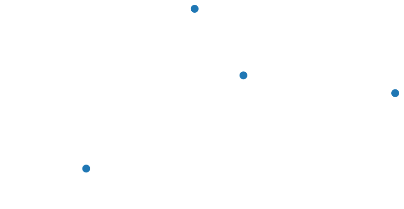
Compared to vega-lite, this is obviously much more verbose, and the resulting plot is just a bare collection of points without axes or axis labels. The vega-lite specification would have looked like this:

{
  "$schema": "https://vega.github.io/schema/vega-lite/v4.json",
  "data": {
    "values": [
      {"x": 15, "y": 8},
      {"x": 72, "y": 25},
      {"x": 35, "y": 44},
      {"x": 44, "y": 29}
    ]
  },
  "mark": "circle",
  "encoding": {
    "x": {"field": "x", "type": "quantitative"},
    "y": {"field": "y", "type": "quantitative"}
  }
}

resulting in this plot:

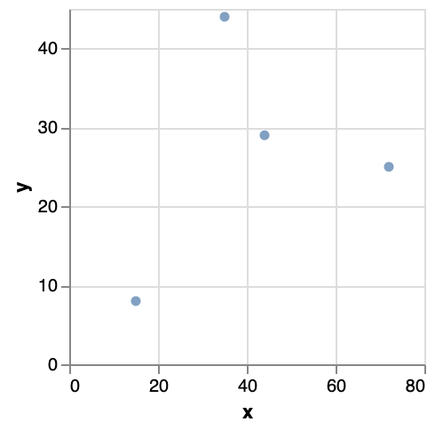
What differences do we see in vega?

• data takes an array instead of a single object
• The mark is a symbol. The default symbol is a circle.
• encoding is moved within marks (now plural instead of the singular mark)
• The encodings include a scale for each element.
• There’s an enter object within encoding.
• In the marks section we need to specify the data used by name.
• We have to define scales that we can use in the encoding.

Changing colour

The points in the plot above are blue. In vega-lite, we’d just add "color": {"value": "red"} to the encoding section to change this. In vega, however, the keyword color is not recognised. Instead, a distinction is made between fill and stroke. fill corresponds to the area of the point itself; stroke refers to the outline of the point (the circle).

Exercise - Change the colour of the points to red.

Exercise - Change the colour of the point outline to green.

Exercise - In the previous exercise, you’ll see that the outline is very thin. Check the documentation for a symbol at https://vega.github.io/vega/docs/marks/symbol/ to find out how to make this line thicker.

Exercise - Change the shape of the symbol from a circle to a square. Again: check the documentation.

Exercise - Let’s try to have to colour of each point dependent on the data itself. Change the data so that each datapoint also has some colour assigned to it (e.g. {"x": 15, "y": 8, "c": "yellow"},) and adjust the encoding to use this colour.

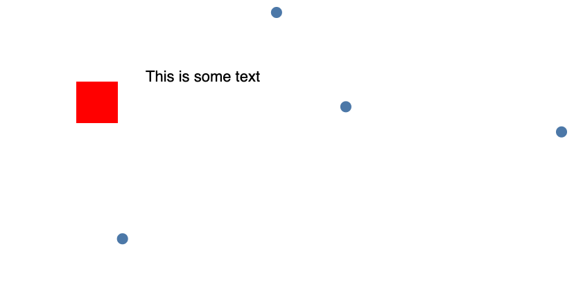
Marks that are not dependent on data

In the marks section in vega, the from pragma points to the dataset that should be used: for every datapoint in the dataset, a single mark is created. If no from is provided, vega defaults to creating a single mark. Let’s for example add a red square to the plot above:

{
  "$schema": "https://vega.github.io/schema/vega/v5.json",
  "width": 400,
  "height": 200,
  "padding": 5,

  "data": [
    {
      "name": "table",
      "values": [
        {"x": 15, "y": 8},
        {"x": 72, "y": 25},
        {"x": 35, "y": 44},
        {"x": 44, "y": 29}
      ]
    }
  ],

  "scales": [
    {
      "name": "xscale",
      "domain": {"data": "table", "field": "x"},
      "range": "width"
    },
    {
      "name": "yscale",
      "domain": {"data": "table", "field": "y"},
      "range": "height"
    }
  ],

  "marks": [
    {
      "type": "symbol",
      "from": {"data":"table"},
      "encode": {
        "enter": {
          "x": {"scale": "xscale", "field": "x"},
          "y": {"scale": "yscale", "field": "y"}
        }
      }
    },
    {
      "type": "rect",
      "encode": {
        "enter": {
          "x": {"value": 50},
          "y": {"value": 50},
          "width": {"value": 30},
          "height": {"value": 30},
          "fill": {"value": "red"}
        }
      }
    },
    {
      "type": "text",
      "encode": {
        "enter": {
          "text": {"value": "This is some text"},
          "x": {"value": 100},
          "y": {"value": 50}
        }
      }
    }
  ]
}

Notice that there is no from defined for the square and the text.

Scales

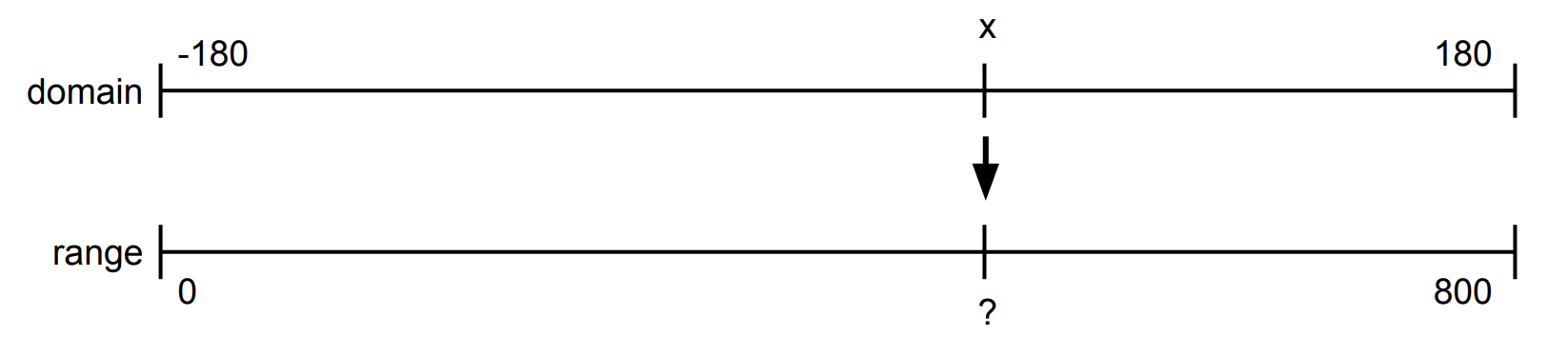
Scales (see their documentation here) convert data from the original domain to a range that can be used for plotting. For example, imagine you have longitude data from a map. Locations on the earth have a longitude that is between -180 and 180. We want to plot this on a graph that is 800 pixels wide. If we’d just use the longitude for the x value, than any location west of Greenwich would be outside of the plot (because smaller than zero), and most of the right of the graphic would be empty (because there are no points in the range -180 to 800). We need to recalculate the positions: -180 (degrees) needs to become 0 (pixels), 0 (degrees) needs to become 400 (pixels) and 180 (degrees) needs to become 800 (pixels).

The most important keys for a scale are its domain and its range. The domain is the original space; the range is the target range. In the case of the longitude data:

A scale also needs to have a name so that it can be referenced later. This is what the most simple scale for the conversion of looks like:

{
  "name": "myscale",
  "type": "linear",
  "domain": [-180,180],
  "range": [0,800]
},

The linear type of scale interpolates the target value linearly. The domain provides the minimum and maximum values of the source values; the range provides the minimum and maximum of the target values. To use this scale, we reference it in the encoding: "x": {"scale": "myscale", "field": "longitude"}.

Instead of providing a minimum and maximum value for domain or range, we can also provide just a single number which is then considered the maximum. This is what you see in the example above for xscale: "range": "width".

Different types of scales exist, including linear, sqrt, ordinal etc. See the documentation at https://vega.github.io/vega/docs/scales/#types for a full reference.

Scales are not only interesting for recalculating ranges, but they are used to assign colours to categories as well. We’ll come back to those later.

Using colour scales

Categorical colours

In the last exercise, we had to define the colour of each bar in the data itself. It’d be better if we can let vega pick the colour for us instead. This is where colour scales come into play.

Vega helps you in assigning colours to datapoints, using a collection of colouring schemes available at https://vega.github.io/vega/docs/schemes/. Instead of hard-coding the colour for each datapoint, let’s give each datapoint a category instead and create a scale to assign colours.

{
  "$schema": "https://vega.github.io/schema/vega/v5.json",
  "width": 400,
  "height": 200,
  "padding": 5,

  "data": [
    {
      "name": "table",
      "values": [
        {"x": 15, "y": 8, "category": "A"},
        {"x": 72, "y": 25, "category": "B"},
        {"x": 35, "y": 44, "category": "C"},
        {"x": 44, "y": 29, "category": "A"},
        {"x": 24, "y": 20, "category": "B"}
      ]
    }
  ],

  "scales": [
    {
      "name": "xscale",
      "domain": {"data": "table", "field": "x"},
      "range": "width"
    },
    {
      "name": "yscale",
      "domain": {"data": "table", "field": "y"},
      "range": "height"
    },
    {
      "name": "colourScale",
      "type": "ordinal",
      "domain": {"data": "table", "field": "category"},
      "range": {"scheme": "category10"}
    }
  ],

  "marks": [
    {
      "type": "symbol",
      "from": {"data":"table"},
      "encode": {
        "enter": {
          "x": {"scale": "xscale", "field": "x"},
          "y": {"scale": "yscale", "field": "y"},
          "size": {"value": 200},
          "fill": {"scale": "colourScale", "field": "category"}
        }
      }
    }
  ]
}

What we did here:

• We added a “category” to each datapoint. This does not have to be named “category”, but can have any name.
• We created a new scale, called “colourScale”. The name, type and domain are as we described above, but for the range we set {"scheme": "category10"}. category10 is only one of the possible colour schemes, which are all listed on https://vega.github.io/vega/docs/schemes/.
• For fill we now use the scale as well.
• Just to make the colour a bit more clear, we increased the size of the points as well…

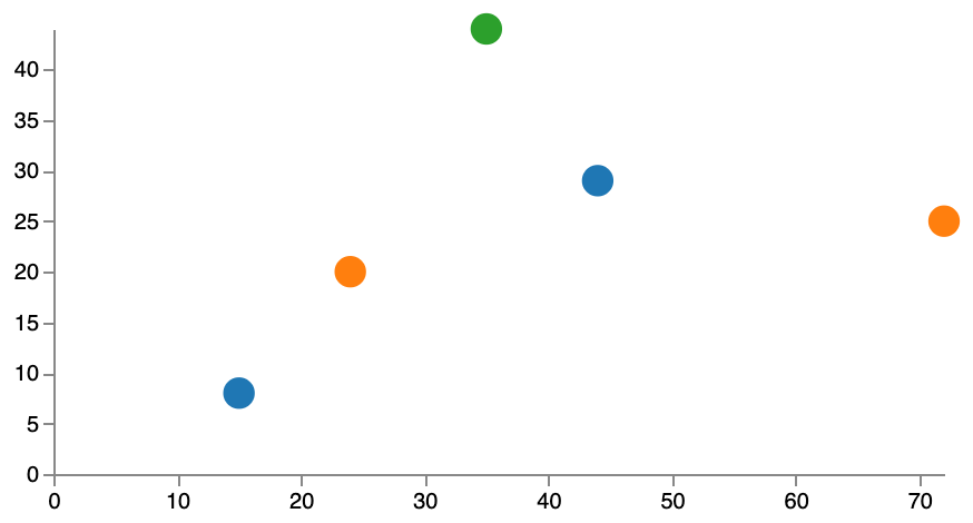
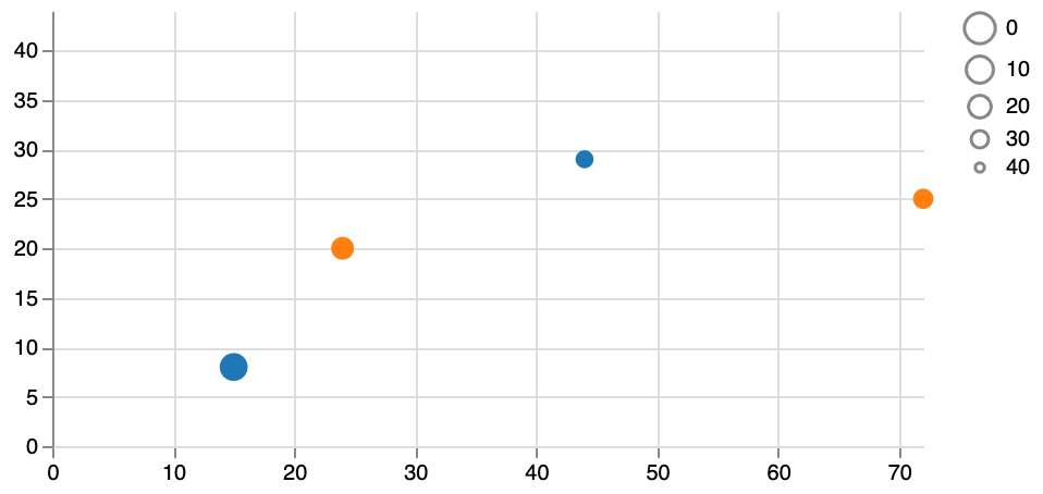
The resulting plot:

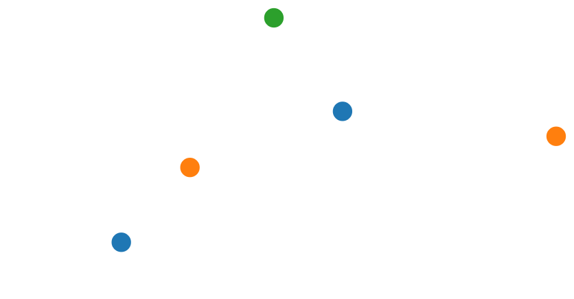
As you can see, the points with the same category get the same colour.

Sequential colours

What if we’d want to have the colour depend not on a nominal value such as category, but on a numerical value? Let’s say, on x.

Change the colourScale to:

{
  "name": "colourScale",
  "type": "linear",
  "domain": {"data": "table", "field": "x"},
  "range": {"scheme": "blues"}
}

and change the field in encoding -> fill from category to x.

You’ll get this image:

Exercise - We use x both in the definition of colourScale and as the field in the encoding. What would it mean if we’d use x in the definition of colourScale, but y in the encoding?

Exercise - Try out some of the diverging colour schemes mentioned on https://vega.github.io/vega/docs/schemes/.

If you really want to, you can also set the colours by hand. For example, we want to have categories A and B be blue, and category C be red. To do this, we simply provide an array both for domain and range, like so:

{
  "name": "colourScale",
  "type": "ordinal",
  "domain": ["A","B","C"],
  "range": ["blue","blue","red"]
}

Enter - Update - Exit

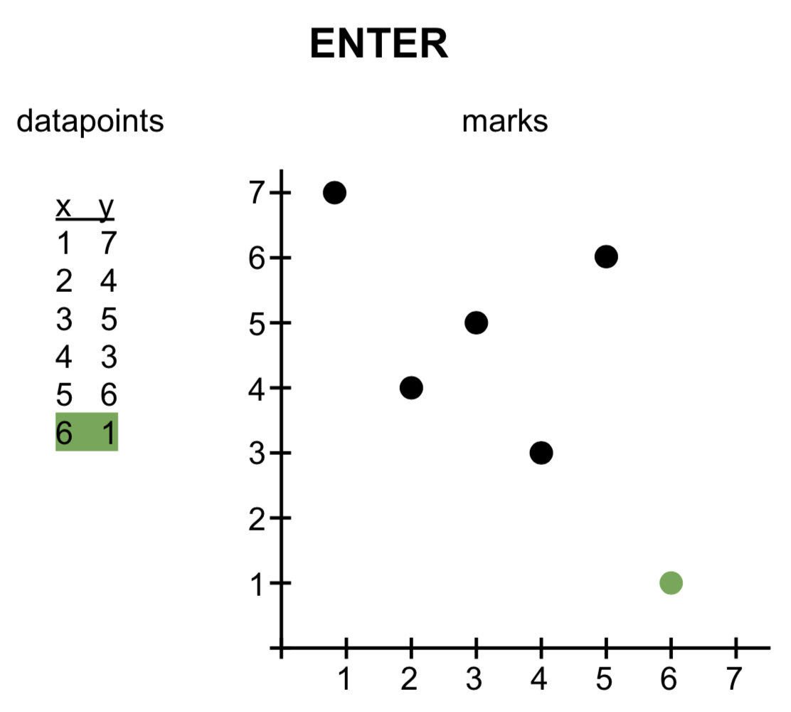
Another difference that we see with vega-lite is the use of the enter tag. This is a very important concept that directly drills down into D3 which is the javascript library underneath vega. To understand the concept, we need to make a clear distinction between marks on the screen, and the data underneath.

For the explanation below, take the initial state of 5 datapoints represented as 5 marks.

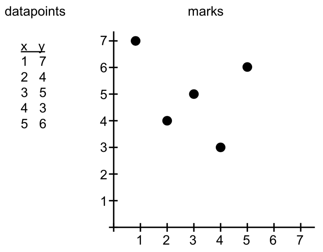
Enter

The enter pragma applies when there are more datapoints than marks on the screen. In the image, a new datapoint [6,1] is created, for which no mark exists yet. The visual encoding that should be applied to that datapoint is defined in the encoding -> enter section.

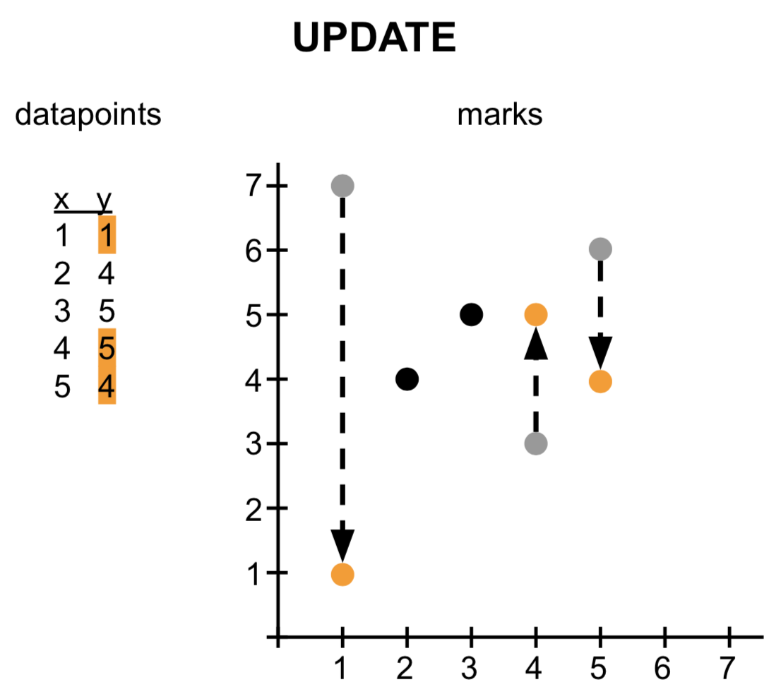
Update

Now let’s change the value some of the datapoints. When the number of marks does not have to change, but they do not represent the correct data anymore, we apply an update (specified in the encoding -> update section). In the image below, it is the y-position that changed, but that might also be color, shape, size, etc of the mark.

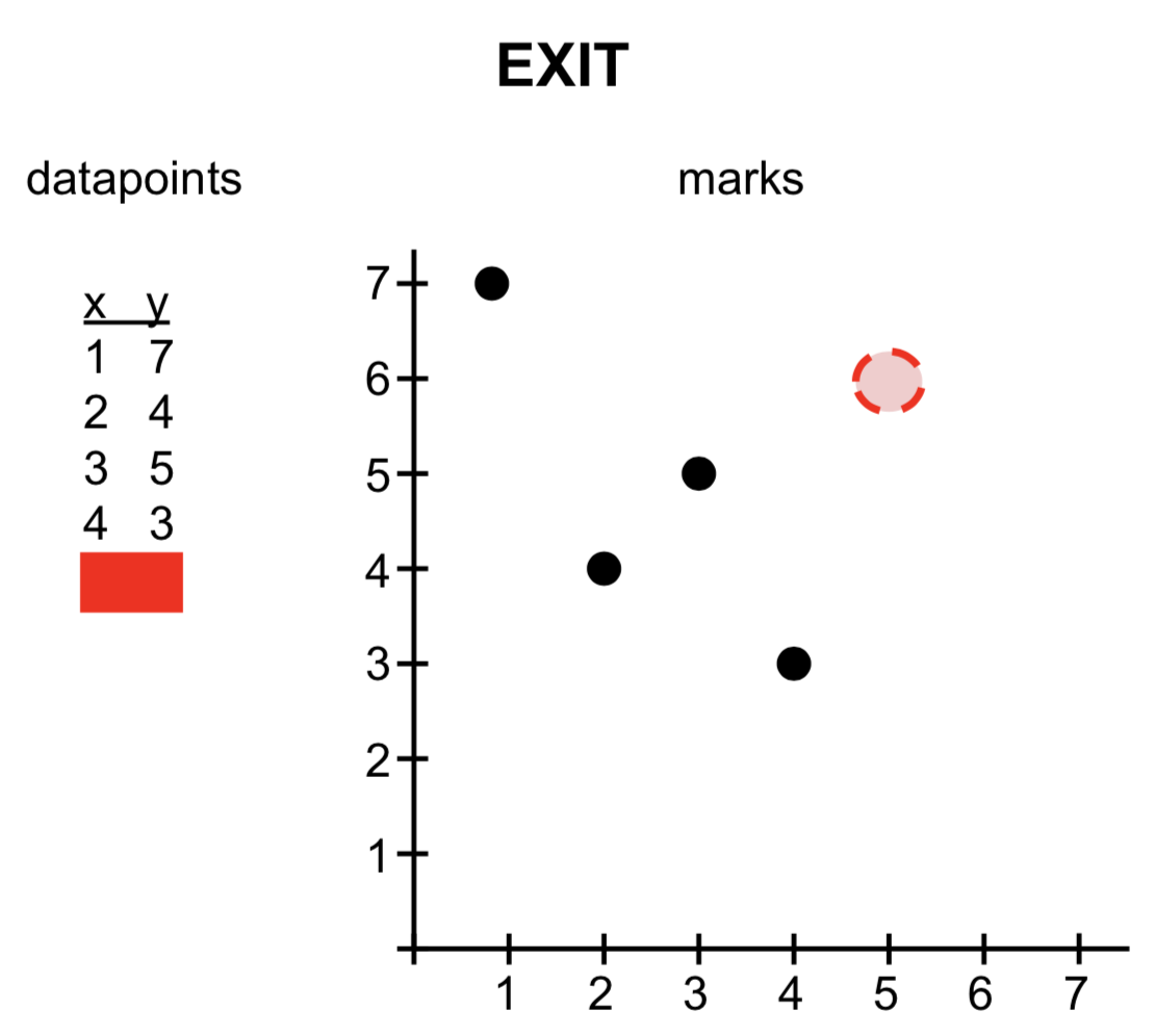
Exit

If after a change in the data there are more marks on the screen than necessary for showing the data (e.g. we go from 5 datapoints to 4), what should happen with the one mark that is still on the screen? It’ll be left hanging, unless we actually remove it. That is what the encoding -> exit section is for.

In the scatterplots above, only the enter is provided, because this is a static dataset that does not change over time (not even changing colour on hover). In other words: we start with a dataset with n datapoints, but no marks yet on the screen. Hence we need the enter.

Axes

The current plot is still extremely bare, without any axes. So let’s add those. See https://vega.github.io/vega/docs/axes/ for documentation.

To add axes to this plot, we merely add the following just before the marks section:

...
"scales": ...,
"axes": [
  {"orient": "bottom", "scale": "xscale"},
  {"orient": "left", "scale": "yscale"}
],
"marks": ...
...

This will give you the following:

For axes, you must provide the orientation (whether top, bottom, left or right), and the scale that decides where the ticks should come.

Exercise - Add these axes to your plot, but also add axis titles and grid lines.

Legends

We now have a plot with points in different colours that are dependent upon the category, but we can’t tell which colour is which category. Enter legends.

By default, a legend is placed in the top right. In our code above, we set the colour (fill) based on the scale colourScale. It is this scale that we need to make a legend for:

"legends": [
  {
    "fill": "colourScale"
  }
],

We used fill because it corresponds to the encoding pragma that we need the legend for, and colourScale because that is the scale that we used in the encoding.

Of course there are other types of legends as well. Let’s for example change "size": {"value": 200} to "size": {"scale": "yscale", "field": "y"}. Our legend would then be:

"legends": [
  {
    "size": "yscale"
  }
],

But wait… This doesn’t look right. We’d expect that points with a larger value for y are larger, and that to be true for the legend as well. It seems that the yscale is the wrong way around. Also, we’ve lost a datapoint!

A solution to this is to create a second scale (e.g. yscalereversed) and use that one for the size and the legend. We’ll still use the original yscale for the position along the Y-axis.

{
  "$schema": "https://vega.github.io/schema/vega/v5.json",
  "width": 400,
  "height": 200,
  "padding": 5,

  "data": [
    {
      "name": "table",
      "values": [
        {"x": 15, "y": 8, "category": "A"},
        {"x": 72, "y": 25, "category": "B"},
        {"x": 35, "y": 44, "category": "C"},
        {"x": 44, "y": 29, "category": "A"},
        {"x": 24, "y": 20, "category": "B"}
      ]
    }
  ],

  "scales": [
    {
      "name": "xscale",
      "domain": {"data": "table", "field": "x"},
      "range": "width"
    },
    {
      "name": "yscale",
      "domain": {"data": "table", "field": "y"},
      "range": "height"
    },
        {
      "name": "yscalereversed",
      "domain": {"data": "table", "field": "y"},
      "range": "height",
      "reverse": true
    },
    {
      "name": "colourScale",
      "type": "ordinal",
      "domain": {"data": "table", "field": "category"},
      "range": {"scheme": "category10"}
    }
  ],
  "axes": [
    {"orient": "bottom", "scale": "xscale", "grid": true},
    {"orient": "left", "scale": "yscale", "grid": true}
  ],
  "legends": [
    {
      "size": "yscalereversed"
    }
  ],
  "marks": [
    {
      "type": "symbol",
      "from": {"data":"table"},
      "encode": {
        "enter": {
          "x": {"scale": "xscale", "field": "x"},
          "y": {"scale": "yscale", "field": "y"},
          "size": {"scale": "yscalereversed", "field": "y"},
          "fill": {"scale": "colourScale", "field": "category"}
        }
      }
    }
  ]
}

This looks more like what we expect:

Why did we loose that datapoint? That’s because the scale went from 0 to the height. The datapoint {"x": 15, "y": 8, "category": "A"} has a value of 8 (which is the smallest value), so it’s mapped to one extreme of the scale. The datapoint {"x": 35, "y": 44, "category": "C"} (which is the largest value) is mapped to the other extreme.

Loading external data

As much as it’s easy, it can become unwieldy to have the actual dataset entered into the vega specification itself. As with vega-lite, we can let vega load data from an external URL. There are some differences with vega-lite, though:

• In vega-lite, the data pragma takes an object ({}) as its value; in vega, it is an array ([]).
• In vega, we need to give a dataset a name.

To re-iterate, here’s the data section that we have been using thus far:

"data": [
  {
    "name": "table",
    "values": [
      {"x": 15, "y": 8, "category": "A"},
      {"x": 72, "y": 25, "category": "B"},
      {"x": 35, "y": 44, "category": "C"},
      {"x": 44, "y": 29, "category": "A"},
      {"x": 24, "y": 20, "category": "B"}
    ]
  }
],

We can load data from a URL like this:

"data": [
  {
    "name": "cars",
    "url": "https://raw.githubusercontent.com/vega/vega/master/docs/data/cars.json"
  }
],

Here is a minimal scatterplot using this car data:

{
  "$schema": "https://vega.github.io/schema/vega/v5.json",
  "width": 400,
  "height": 200,
  "padding": 5,

  "data": [
    {
      "name": "cars",
      "url": "https://raw.githubusercontent.com/vega/vega/master/docs/data/cars.json"
    }
  ],

  "scales": [
    {
      "name": "xscale",
      "domain": {"data": "cars", "field": "Acceleration"},
      "range": "width"
    },
    {
      "name": "yscale",
      "domain": {"data": "cars", "field": "Miles_per_Gallon"},
      "range": "height"
    }
  ],
  "axes": [
    {"orient": "bottom", "scale": "xscale", "grid": true},
    {"orient": "left", "scale": "yscale", "grid": true}
  ],
  "marks": [
    {
      "type": "symbol",
      "from": {"data":"cars"},
      "encode": {
        "enter": {
          "x": {"scale": "xscale", "field": "Acceleration"},
          "y": {"scale": "yscale", "field": "Miles_per_Gallon"}
        }
      }
    }
  ]
}

The result:

Exercise - Add a plot title, legend and axis titles to this plot, and make the dots more transparent so that we can see where points are plotted on top of each other. It should look like this: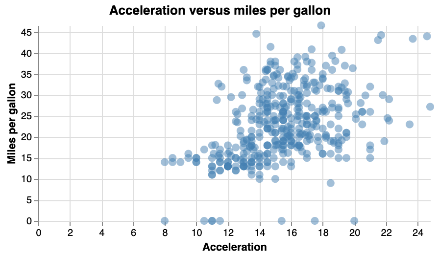

Exercise - Take the previous plot, and colour the points based on “Origin” (i.e. continent). Add a legend to show which colour corresponds to which origin. (First take a look at the data itself at the URL to know what it looks like.) The plot should look like this: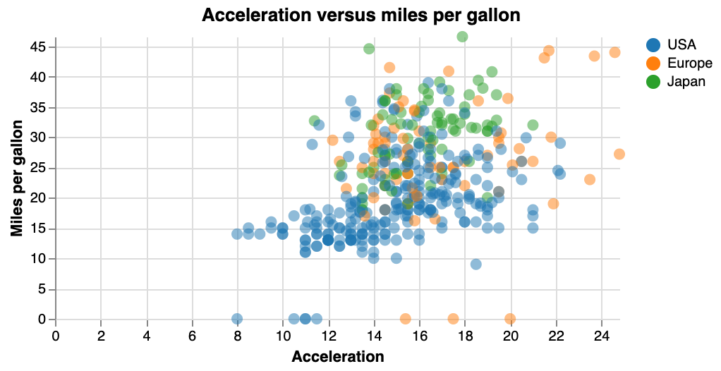

Transforms

In the vega-lite tutorial, we saw how we can use transforms to preprocess the data before it gets plotted. We can filter the data, aggregate it, compute a formula, sample, etc. For a full list of possible transformations, see the transform documentation at https://vega.github.io/vega/docs/transforms/.

As we can define different datasets in vega (which is not possible in vega-lite), we can independently define different subsets of the data, or aggregations.

Creating a subset of the data just for the European cars, we can do the following:

"data": [
  {
    "name": "cars",
    "url": "https://raw.githubusercontent.com/vega/vega/master/docs/data/cars.json"
  },
  {
    "name": "euro-cars",
    "source": "cars",
    "transform": [
      {"type": "filter", "expr": "datum.Origin == 'Europe'"}
    ]
  }
]

This creates the cars dataset as we had before, but also a subset of European cars.

Exercise - How would we now use this filtered dataset for the marks? Make an acceleration versus mpg plot for only the european cars.

We can do the same for aggregation to create a histogram. Whereas the original data is not available anymore in vega-lite, it can still be in vega.

...
"data": [
  {
    "name": "cars",
    "url": "https://raw.githubusercontent.com/vega/vega/master/docs/data/cars.json"
  },
  {
    "name": "binned",
    "source": "cars",
    "transform": [
      {"type": "bin", "field": "Acceleration", "extent": [0,25]}
    ]
  },
  {
    "name": "aggregated",
    "source": "binned",
    "transform": [
      {"type": "aggregate",
        "key": "bin0", "groupby": ["bin0", "bin1"],
        "fields": ["bin0"], "ops": ["count"], "as": ["count"]}
    ]
  }
],
...

There are now three different datasets available: cars, binned and aggregated. We can have each separate like this, or - as we don’t expect to ever use the binned dataset by itself, merge binned and aggregated like we had to do in vega-lite anyway:

...
"data": [
  {
    "name": "cars",
    "url": "https://raw.githubusercontent.com/vega/vega/master/docs/data/cars.json"
  },
  {
    "name": "aggregated",
    "source": "cars",
    "transform": [
      {"type": "aggregate",
        "key": "bin0", "groupby": ["bin0", "bin1"],
        "fields": ["bin0"], "ops": ["count"], "as": ["count"]},
      {"type": "bin", "field": "Acceleration", "extent": [0,25]}
    ]
  }
],
...

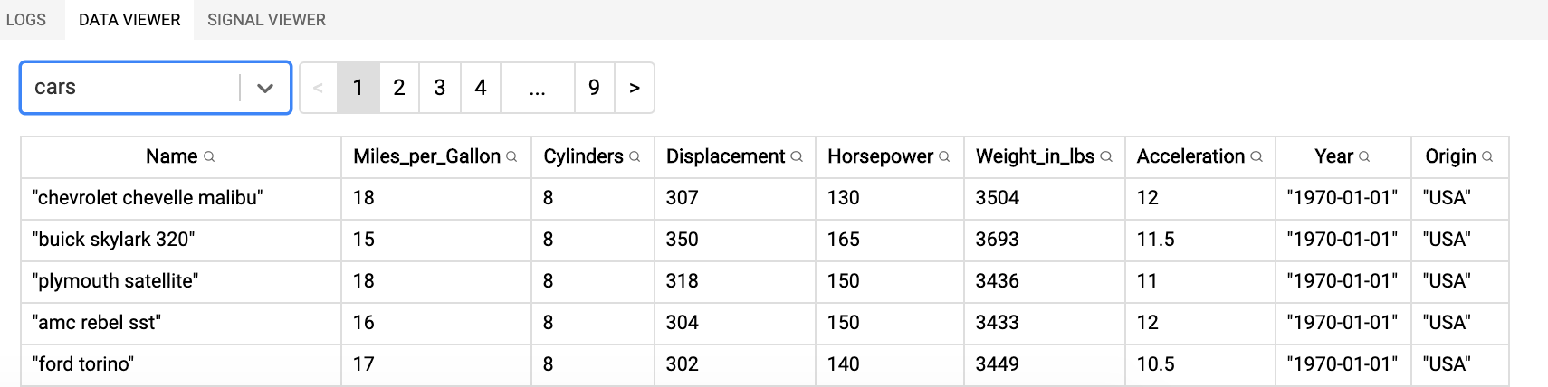
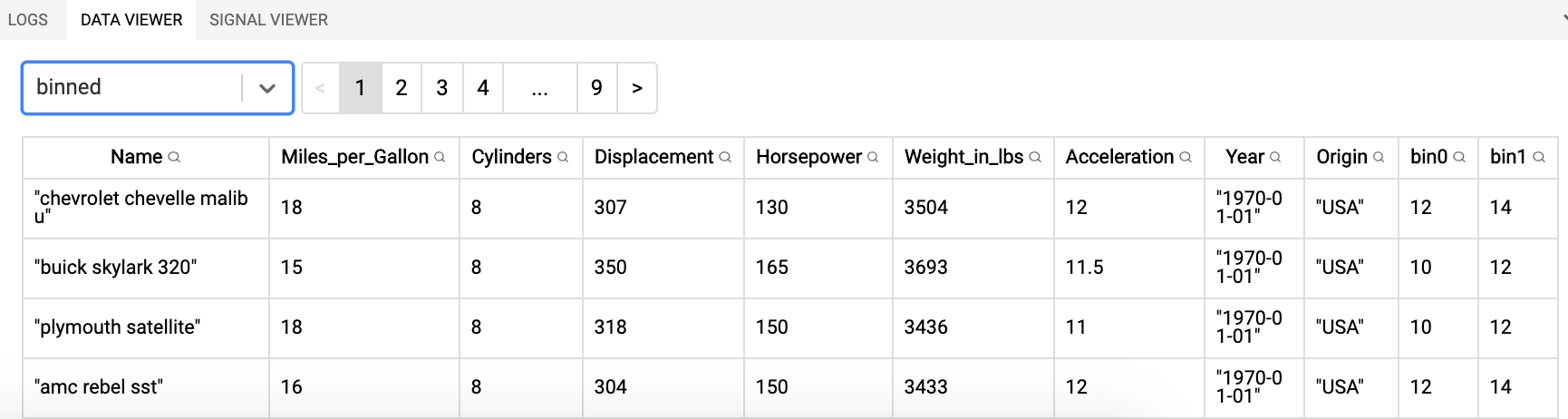
Important tip: when using the vega editor at https://vega.github.io/editor, have a look at the data viewer in the lower-right corner: it shows you what each of the datasets looks like.

The original dataset:

The binned dataset (note the two additional columns at the end):

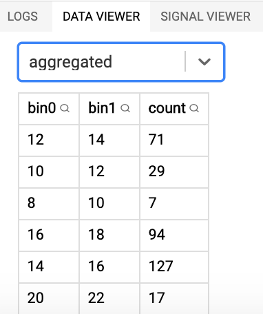
The aggregated dataset:

Interaction

Simple interaction

You do get some interaction for free with vega, including tooltips, effects on hover, etc.

To add a simple tooltip, just add that pragma to the marks, for example:

...
"marks": [
  {
    "type": "symbol",
    "from": {"data":"cars"},
    "encode": {
      "enter": {
        "x": {"scale": "xscale", "field": "Acceleration"},
        "y": {"scale": "yscale", "field": "Miles_per_Gallon"},
        "tooltip": {"field": "Name"}
      }
    }
  }
]
...

This will show the name of the car when you hover over a point.

Exercise - Implement this.

You can change the visual encoding of a mark when hovering over it, using code like this:

...
"marks": [
  {
    "type": "symbol",
    "from": {"data":"cars"},
    "encode": {
      "enter": {
        "x": {"scale": "xscale", "field": "Acceleration"},
        "y": {"scale": "yscale", "field": "Miles_per_Gallon"},
        "tooltip": {"field": "Name"}
      },
      "update": {
        "fill": {"value": "steelblue"},
        "fillOpacity": {"value": 0.3},
        "size": {"value": 100}
      },
      "hover": {
        "fill": {"value": "red"},
        "fillOpacity": {"value": 1},
        "size": {"value": 500}
      }
    }
  }
]
...

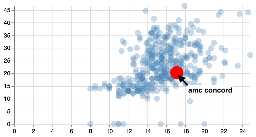
The result:

Advanced interaction

Vega uses the reactive paradigm for interactivity. It’s a bit like cells in an Excel sheet that change dynamically if any of the referenced cells change value: like a cell that has the formula =SUM(A3:A5) which value changes when we enter a new value in cell A3.

The OpenVis talk at https://www.youtube.com/watch?v=Y8Fp9z-9DWc describes the system in detail. Much of the following is taken from that talk, and the underlying paper. See also Satyanarayan’s UIST talk.

In the static images we created above, we had to define the data, transforms, scales, guides and marks. Similarly, the following concepts apply when talking about interaction.

Static	Dynamic	Example
data	event streams	[mousedown, mouseup] > mousemove
transforms	signals	minX = min(width, event.x)
scales	scale inversions	minVal = xScale.invert(minX)
guides	predicates	p(t) = minVal =< t.value =< maxVal
marks	production rules	fill = p(t) -> colorScale(t.category) ; nil -> grey

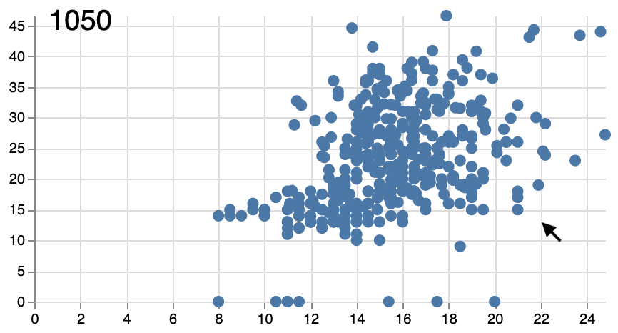
Event streams

As per the documentation: “Event streams are the primary means of modelling user input to enable dynamic, interactive visualisations. Event streams capture a sequence of input events such as mouse click, touch movement, timer ticks, or signal updates. When events that match a stream definition occur, they cause any corresponding signal event handlers to evaluate, potentially updating a signal value.”

Events are not described in their separate section in the vega specification, but within the signals that get triggered when an event happens. For example, the following code makes a signal mouseX available which is updated every time the mouse is moved. This signal is then used in the marks section to display that position.

...
"signals": [
  {
    "name": "mouseX",
    "on": [
      {"events":"mousemove", "update": "event.x"}
    ]
  }
],
...
"marks": [
  {
    "type": "text",
    "encode": {
      "enter": {
        "x": {"value": 10},
        "y": {"value": 10}
      },
      "update": {
        "text": {"signal": "mouseX"}
      }
    }
  }
]
...

Note that now we have seen 3 different ways to define the value to use for setting parameters:

• "value", e.g. "x": {"value": 10} for fixed values
• "field", e.g. "x": {"field": "Acceleration"} for values that are dependent on the dataset
• "signal", e.g. "x": {"signal": "mouseX"} for values that can change over time

Notice in this code that we put the "text" part within "update" and not within "enter". This is because what is defined in "enter" is only read once. Any parameters that do not change can be put there, though.

Event types that you can use include click, cblclick, dragenter, dragleave, mousedown, mouseup, mousemove, etc. For the full list, see https://vega.github.io/vega/docs/event-streams/.

These event types can be applied to different sources: the screen (e.g. a mousemove on the screen), any mark (e.g. rect:click), or a particular mark (e.g. @mymark:dragenter). Some more examples of event types applied to different sources (again from the documentation):

Event	What it does
mousedown	capture all mousedown events, regardless of source
*:mousedown	mousedown events on marks, but not the view itself
rect:mousedown	mousedown events on any rect marks
@foo:mousedown	mousedown events on marks named ‘foo’
window:mousemove	capture mousemove events from the browser window
timer{1000}	capture a timer tick every 1000 ms
mousemove[event.buttons]	mousemove events with any mouse button pressed
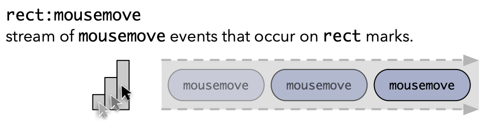
click[event.shiftKey]	click events with the shift key pressed

Combining event streams

Often you will want to filter event streams (e.g. to throttle them so that you only get a signal every 5 seconds or so), or combine them.

A single event stream is defined as described above.

Streams can be filtered so that not all events trigger a signal. In the picture below, the top stream is the original and the bottom stream is the one that gets through to the signal.

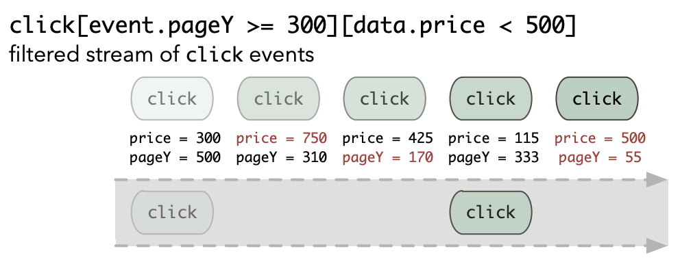
You can also filter events in a stream by whether or not they are between two other events.

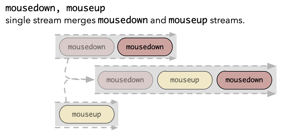
You can merge different streams into one.

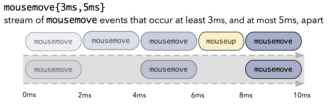
And finally you can also throttle event streams so that only a certain number of events get through in a given period of time.

Signals

So once an event occurs, the corresponding signal changes. In the example above, every time the mouse is moved, the event.x (i.e. the horizontal position on the screen of where the event (i.e. the moving mouse) occurred) is made available to Vega through the mouseX variable/signal.

This mouseX can then be used in the specification for the marks, scales, etc.

Different patterns for signals:

{
  "name": "colourSelector",
  "bind": {"input": "select", "options": ["steelblue","red"]
}

{
  "name": "mouseX",
  "on": [ {"events":"mousemove", "update": "event.x"} ]
}

TODO: others?

Using widgets to set signals

Sometimes it’d be nice to make a plot interactive so that you can set parameters without having to dive into the vega specification. We can use signals for this.

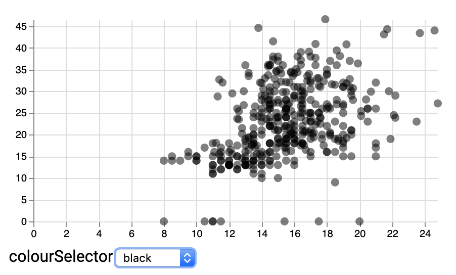
Setting colour using a dropdown box

We can create a “colourSelector” signal (the name is arbitrary), which is bound to an input widget using "bind": {"input": "select", "options": ["black","steelblue","red"]}. The default value can be set in the signals pragma itself as well. In the mark encoding, we can set "fill": {"signal": "colourSelector"}. But make sure to do this in an update section and not in enter, as this value will change.

{
  "$schema": "https://vega.github.io/schema/vega/v5.json",
  "width": 400,
  "height": 200,
  "padding": 5,

  "data": [
    {
      "name": "cars",
      "url": "https://raw.githubusercontent.com/vega/vega/master/docs/data/cars.json"
    }
  ],
  "signals": [
    {
      "name": "colourSelector",
      "bind": {"input": "select", "options": ["black","steelblue","red"]},
      "value": "red"
    }
  ],
  "scales": [
    {
      "name": "xscale",
      "domain": {"data": "cars", "field": "Acceleration"},
      "range": "width"
    },
    {
      "name": "yscale",
      "domain": {"data": "cars", "field": "Miles_per_Gallon"},
      "range": "height"
    }
  ],
  "axes": [
    {"orient": "bottom", "scale": "xscale", "grid": true},
    {"orient": "left", "scale": "yscale", "grid": true}
  ],
  "marks": [
    {
      "type": "symbol",
      "from": {"data":"cars"},
      "encode": {
        "enter": {
          "x": {"scale": "xscale", "field": "Acceleration"},
          "y": {"scale": "yscale", "field": "Miles_per_Gallon"},
          "fillOpacity": {"value": 0.5}
        },
        "update": {
          "fill": {"signal": "colourSelector"}
        }
      }
    }
  ]
}

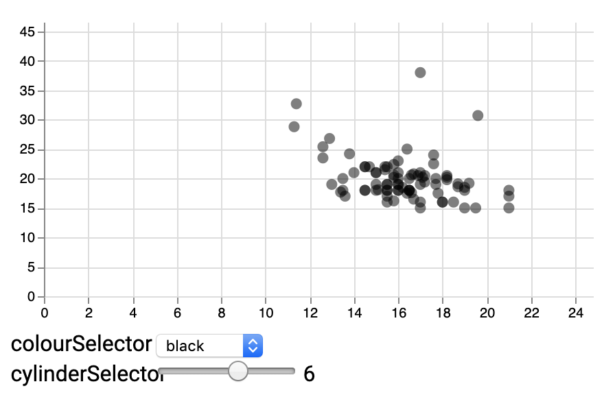
Selecting a value using a slider

We can also hide the datapoints that do not comply to a given filter, e.g. on number of cylinders:

{
  "$schema": "https://vega.github.io/schema/vega/v5.json",
  "width": 400,
  "height": 200,
  "padding": 5,

  "data": [
    {
      "name": "cars",
      "url": "https://raw.githubusercontent.com/vega/vega/master/docs/data/cars.json"
    }
  ],
  "signals": [
    {
      "name": "colourSelector",
      "bind": {"input": "select", "options": ["black","steelblue","red"]},
      "value": "red"
    },
    {
      "name": "cylinderSelector",
      "bind": {"input": "range", "min": 3, "max": 8, "step": 1},
      "value": 4
    },
    {
      "name": "test"
    }
  ],
  "scales": [
    {
      "name": "xscale",
      "domain": {"data": "cars", "field": "Acceleration"},
      "range": "width"
    },
    {
      "name": "yscale",
      "domain": {"data": "cars", "field": "Miles_per_Gallon"},
      "range": "height"
    }
  ],
  "axes": [
    {"orient": "bottom", "scale": "xscale", "grid": true},
    {"orient": "left", "scale": "yscale", "grid": true}
  ],
  "marks": [
    {
      "type": "symbol",
      "from": {"data":"cars"},
      "encode": {
        "enter": {
          "x": {"scale": "xscale", "field": "Acceleration"},
          "y": {"scale": "yscale", "field": "Miles_per_Gallon"}
        },
        "update": {
          "fillOpacity": {"signal": "datum.Cylinders == cylinderSelector ? 0.5 : 0"},
          "fill": {"signal": "colourSelector"}
        }
      }
    }
  ]
}

Exercise - In the Transform section above, we created a filtered dataset containing only European cars. This dataset was called euro-cars. We could do the same for American and Japanese cars, calling them us-cars and japanese-cars. To actually use one of these more specific datasets for the marks, we had to change "from": {"data":"cars"} to "from": {"data":"euro-cars"} in the code. Although this is good for when you’re developing your visualisation, it’d be much better if we didn’t have to dive into the code just to select the dataset. Create a dropdown box that let’s you choose which of the three regions of origin to choose, using the fillOpacity trick we used above.

Exercise - Now try to do the same thing where, instead of using this opacity trick, you actually define a filtered dataset that contains only the data for the region that you select using the dropdown box.

Composing plots

Remember in vega-lite that we could create composed plots by using concat, hconcat or vconcat. Vega is more powerful to create layouts involving different plots. However, it is much more difficult/verbose to do so…

In the vega-lite tutorial, we created a double scatterplot for the cars data, that looked like this:

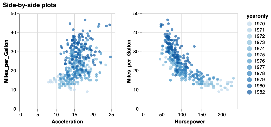
If we want to recreate this using vega, here is the minimal specification:

{
  "$schema": "https://vega.github.io/schema/vega/v5.json",
  "padding": 5,
  "data": [
    {
      "name": "cars",
      "url": "https://raw.githubusercontent.com/vega/vega/master/docs/data/cars.json",
      "format": {"type": "json"}
    }
  ],
  "scales": [
    {
      "name": "acceleration_xscale",
      "type": "linear",
      "domain": {"data": "cars", "field": "Acceleration"},
      "range": [0, 200],
      "nice": true,
      "zero": true
    },
    {
      "name": "mpg_yscale",
      "type": "linear",
      "domain": {"data": "cars", "field": "Miles_per_Gallon"},
      "range": [200, 0],
      "nice": true,
      "zero": true
    },
    {
      "name": "horsepower_xscale",
      "type": "linear",
      "domain": {"data": "cars", "field": "Horsepower"},
      "range": [0, 200],
      "nice": true,
      "zero": true
    }
  ],
  "layout": {"padding": 20},
  "marks": [
    {
      "type": "group",
      "encode": {
        "update": {
          "width": {"value": 200},
          "height": {"value": 200}
        }
      },
      "marks": [
        {
          "type": "symbol",
          "style": "circle",
          "from": {"data": "cars"},
          "encode": {
            "update": {
              "x": {"scale": "acceleration_xscale", "field": "Acceleration"},
              "y": {"scale": "mpg_yscale", "field": "Miles_per_Gallon"},
              "fill": {"value": "steelblue"},
              "fillOpacity": {"value": 0.5}
            }
          }
        }
      ],
      "axes": [
        {
          "scale": "mpg_yscale",
          "orient": "left",
          "gridScale": "mpg_yscale",
          "grid": true,
          "tickCount": 5,
          "title": "Miles_per_Gallon"
        },
        {
          "scale": "acceleration_xscale",
          "orient": "bottom",
          "gridScale": "acceleration_xscale",
          "grid": true,
          "tickCount": 5,
          "title": "Acceleration"
        }
      ]
    },
    {
      "type": "group",
      "style": "cell",
      "encode": {
        "update": {
          "width":  {"value": 200},
          "height": {"value": 200}
        }
      },
      "marks": [
        {
          "type": "symbol",
          "style": "circle",
          "from": {"data": "cars"},
          "encode": {
            "enter": {
              "x": {"scale": "horsepower_xscale", "field": "Horsepower"},
              "y": {"scale": "mpg_yscale", "field": "Miles_per_Gallon"},
              "fill": {"value": "steelblue"},
              "fillOpacity": {"value": 0.5}
            }
          }
        }
      ],
      "axes": [
        {
          "scale": "mpg_yscale",
          "orient": "left",
          "gridScale": "mpg_yscale",
          "grid": true,
          "tickCount": 5,
          "title": "Miles_per_Gallon"
        },
        {
          "scale": "horsepower_xscale",
          "orient": "bottom",
          "gridScale": "horsepower_xscale",
          "grid": true,
          "tickCount": 5,
          "title": "Horse power"
        }
      ]
    }
  ]
}

For simplicity’s sake, we left out the colourScale and legend. Still, the specification is huge: 125 lines versus what would have taken 23 lines in vega-lite.

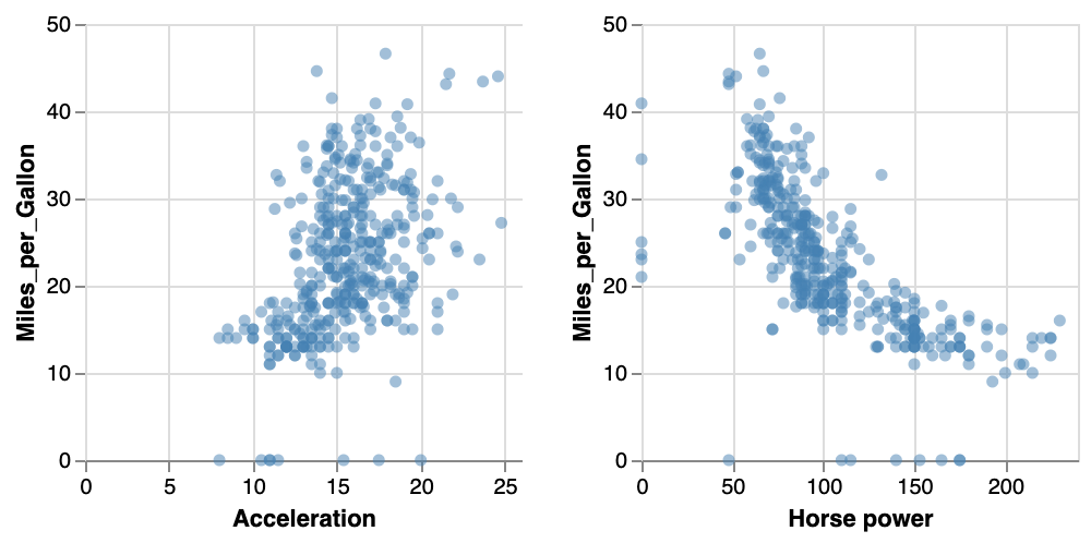
In vega, we need to set the layout, and the marks is itself an array of subplots (each containing another marks…).

Brushing and linking

Whereas brushing and linking in vega-lite is very simple to do, it is very hard in vega. Although it is possible, you’ll have to play with signals, data, and some non-documented functions within the vega code. Therefore, we won’t go into brushing and linking in this tutorial.

Hopefully, brushing/linking will be easier in one of the next versions.

Advanced transforms

Scatterplots, lineplots, bar charts etc are easy to define: the x and y position on the screen is directly dictated by the data. This is not the case for more advanced layouts such as node-link diagrams for networks, word clouds or voronoi diagrams.

Force-directed layout for networks

Let’s start with a node-link diagram for a network. We’ll use the miserables dataset for this.

Minimal network

Here’s a minimal vega specification, without colours or dragging:

{
  "$schema": "https://vega.github.io/schema/vega/v5.json",
  "width": 350,
  "height": 250,
  "padding": 0,
  "autosize": "none",

  "signals": [
    { "name": "cx", "update": "width / 2" },
    { "name": "cy", "update": "height / 2" }
  ],

  "data": [
    {
      "name": "node-data",
      "url": "https://raw.githubusercontent.com/vega/vega-datasets/master/data/miserables.json",
      "format": {"type": "json", "property": "nodes"}
    },
    {
      "name": "link-data",
      "url": "https://raw.githubusercontent.com/vega/vega-datasets/master/data/miserables.json",
      "format": {"type": "json", "property": "links"}
    }
  ],

  "marks": [
    {
      "name": "nodes",
      "type": "symbol",
      "zindex": 1,

      "from": {"data": "node-data"},

      "encode": {
        "enter": {
          "fill": {"value": "grey"}
        }
      },

      "transform": [
        {
          "type": "force",
          "iterations": 300,
          "velocityDecay": 0.4,
          "forces": [
            {"force": "center", "x": {"signal": "cx"}, "y": {"signal": "cy"}},
            {"force": "collide", "radius": 5},
            {"force": "nbody", "strength": -10},
            {"force": "link", "links": "link-data", "distance": 15}
          ]
        }
      ]
    },
    {
      "type": "path",
      "from": {"data": "link-data"},
      "interactive": false,
      "encode": {
        "update": {
          "stroke": {"value": "lightgrey"},
          "strokeWidth": {"value": 0.5}
        }
      },
      "transform": [
        {
          "type": "linkpath", "shape": "line",
          "sourceX": "datum.source.x", "sourceY": "datum.source.y",
          "targetX": "datum.target.x", "targetY": "datum.target.y"
        }
      ]
    }
  ]
}

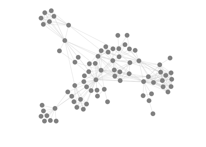
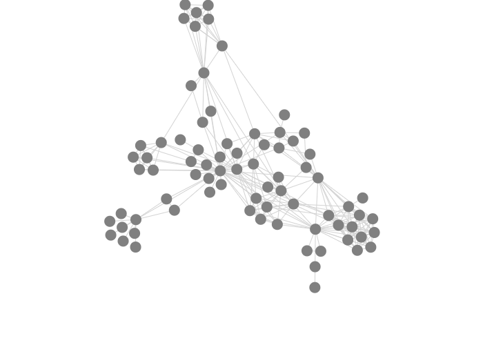
This is what the plot looks like:

Let’s break this down:

• data: If you follow the URL to the JSON file, you’ll see that it looks like this: {nodes: [], links: []}. We create two different datasets: one for the nodes and one for the links. The format.property bit specifies which part needs to be extracted. It would seem that we’d be able to do this using a single dataset and creating two derived ones using source, but unfortunately it’s not possible to extract a single element using a transform.
• marks: There are two types of marks, namely for the nodes and for the edges. In principle, you can draw the nodes without the edges (try it), but not the other way around because the edge positions depend on the source and target nodes.
  • For the nodes, everything is the same as we saw in all our previous exercises, except for the zindex and transform. The "zindex": 1 makes sure that the nodes are drawn on top of the edges.
    • transform: Definitely have a good look at the documentation for this. We use a single transform of type force. Actually, it’s not just one force, but several which we list under "forces": []. The algorithm will try to find an equilibrium between all of these interacting forces.
      • center: Indicates what the center of the plot should be. This would typically be the center of your screen, i.e. width/2 and height/2.
      • collide: To what extent should nodes be pushed apart, but only when they overlap.
      • nbody: To what extent should nodes be pushed apart or attracted. A negative value will push them apart; a positive one will pull them together. This value will have the largest impact on what your plot looks like.
      • link: While nbody will push nodes apart or attract them, this is contrained by the links between them.
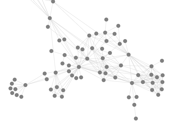
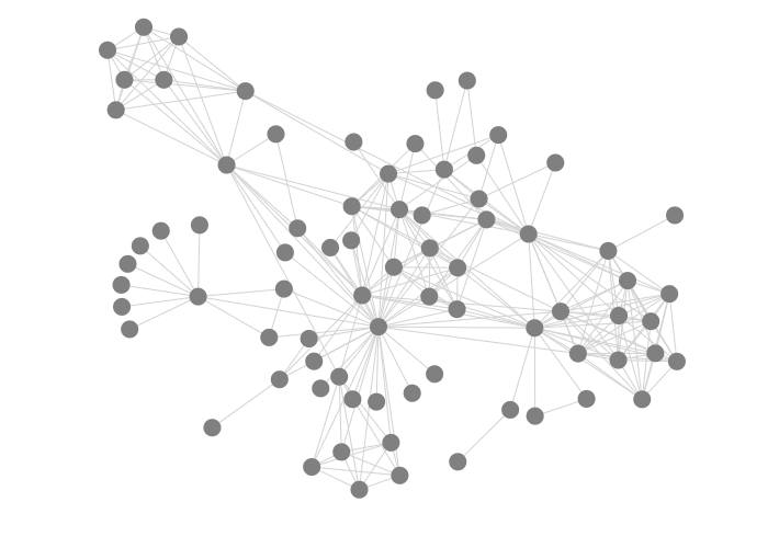
  • For the links, we use path marks instead of line because the first can have arbitrary position, while lines are used for longitudinal data.
    • We set stroke and strokeWidth in an update section instead of enter. If we’d use enter, the paths wouldn’t update when the nodes move around. You’d get a picture like this instead: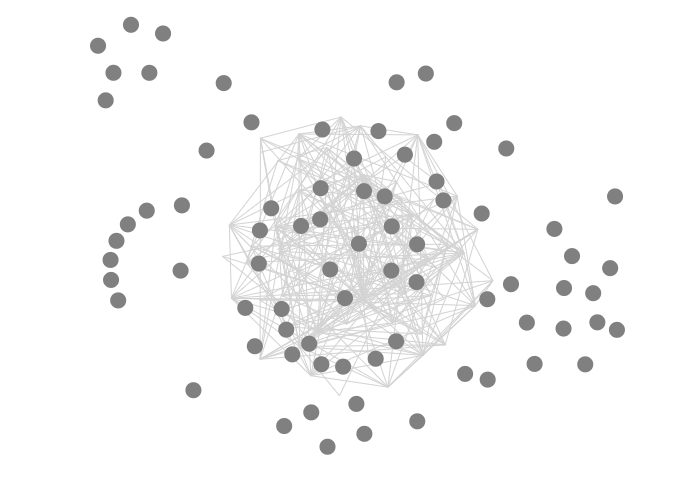
      
    • transform: We use the special linkpath transform, which is specifically for drawing a path between a source and a target. Apart from line, the shape can also be a curve, arc, diagonal or orthogonal. Try these out as well.

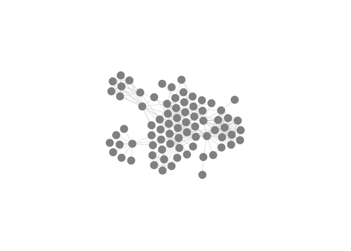
Here are some examples of plots with different settings for collide, nbody and link in the node transform:

Altering collide, with nbody equal to -10 and link equal to 15:

1	5	10

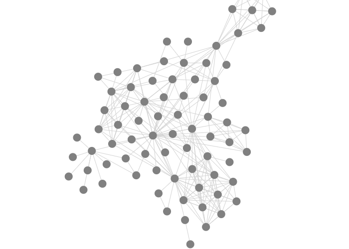Altering nbody, with collide equal to 5 and link equal to 15:

-2	-10	-20

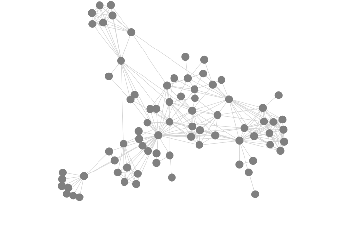
Altering link, with collide equal to 5 and nbody equal to -10:

5	15	30

Exercise - What happens if you change the value of nbody to 1? Or to 10? Does the value of collide have an effect? If so: what effect?

Adding node dragging

Here’s an example where we can drag nodes around:

{
  "$schema": "https://vega.github.io/schema/vega/v5.json",
  "width": 400,
  "height": 275,
  "padding": 0,
  "autosize": "none",

  "signals": [
    { "name": "cx", "update": "width / 2" },
    { "name": "cy", "update": "height / 2" },
    {
      "description": "State variable for active node dragged status.",
      "name": "dragged", "value": 0,
      "on": [
        {
          "events": "symbol:mouseout[!event.buttons], window:mouseup",
          "update": "0"
        },
        {
          "events": "symbol:mouseover",
          "update": "dragged || 1"
        },
        {
          "events": "[symbol:mousedown, window:mouseup] > window:mousemove!",
          "update": "2", "force": true
        }
      ]
    },
    {
      "description": "Graph node most recently interacted with.",
      "name": "dragged_node", "value": null,
      "on": [
        {
          "events": "symbol:mouseover",
          "update": "dragged === 1 ? item() : dragged_node"
        }
      ]
    },
    {
      "description": "Flag to restart Force simulation upon data changes.",
      "name": "restart", "value": false,
      "on": [
        {"events": {"signal": "dragged"}, "update": "dragged > 1"}
      ]
    }
  ],

  "data": [
    {
      "name": "node-data",
      "url": "data/miserables.json",
      "format": {"type": "json", "property": "nodes"}
    },
    {
      "name": "link-data",
      "url": "data/miserables.json",
      "format": {"type": "json", "property": "links"}
    }
  ],

  "marks": [
    {
      "name": "nodes",
      "type": "symbol",
      "zindex": 1,

      "from": {"data": "node-data"},
      "on": [
        {
          "trigger": "dragged",
          "modify": "dragged_node",
          "values": "dragged === 1 ? {fx:dragged_node.x, fy:dragged_node.y} : {fx:x(), fy:y()}"
        },
        {
          "trigger": "!dragged",
          "modify": "dragged_node", "values": "{fx: null, fy: null}"
        }
      ],

      "encode": {
        "enter": {
          "fill": {"value": "grey"}
        },
        "update": {
          "size": {"value": 50},
          "cursor": {"value": "pointer"}
        }
      },

      "transform": [
        {
          "type": "force",
          "iterations": 300,
          "velocityDecay": 0.4,
          "restart": {"signal": "restart"},
          "static": false,
          "forces": [
            {"force": "center", "x": {"signal": "cx"}, "y": {"signal": "cy"}},
            {"force": "collide", "radius": 5},
            {"force": "nbody", "strength": -10},
            {"force": "link", "links": "link-data", "distance": 15}
          ]
        }
      ]
    },
    {
      "type": "path",
      "from": {"data": "link-data"},
      "interactive": false,
      "encode": {
        "update": {
          "stroke": {"value": "lightgrey"}
        }
      },
      "transform": [
        {
          "type": "linkpath", "shape": "line",
          "sourceX": "datum.source.x", "sourceY": "datum.source.y",
          "targetX": "datum.target.x", "targetY": "datum.target.y"
        }
      ]
    }
  ]
}

What has changed?

• A signal dragged captures if anything is dragged. Possible values are: 0 (nothing is being dragged), 1 (on mouseover: something could be dragged) and 2 (something is actually being dragged).
• A signal dragged_node, which is a container for the actual node being dragged. If the value of dragged is 1 (i.e. ready to drag, but not actually dragging yet), the value for dragged_node will be set to item(), which is the element on which an event is active (see here). Why do we actually check for the value of dragged? If you don’t and start dragging a node across another one, it might happen that your mouse picks up another node than the original one on the way.
• A signal restart to ensure that positions of the nodes are recalculated when we drag a node to a new position. Now how does the code {"events": {"signal": "dragged"}, "update": "dragged > 1"} actually work? The signal will fire every time the dragged signal changes. Its update is dragged > 1. dragged > 1 is a test: it returns true or false. It is this true or false that will be stored in the symbol restart.
• A trigger dragged on the nodes changes the dragged_node’s fx and fy. fx and fy are two special fields on a node object, and stand for fixed x and fixed y. If dragged === 1 (i.e. the mouse hovers over the node), fx is set to the x-position of dragged_node and fy accordingly. This is so that the node stays in a fixed position while you’re on top of it and does not escape from under the mouse. If dragged is not 1 (i.e. it’s 2), fx and fy are set to x() and y() which are the x- and y-position of the mouse. So as your mouse moves around, the node will follow.
• A trigger !dragged, which stands for not dragged. When the signal dragged is set to 0, fx and fy are set to null, meaning that the node can participate again in all forces in the network.

Exercise - The individuals in the miserables data belong to different groups. Use these groups to set the colour of the nodes.

Exercise - Create two plots next to each other: one with this network, and one with a histogram of the number of individuals per group. So something like this: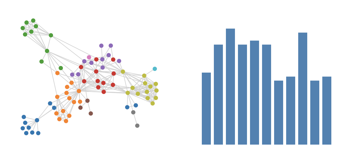

Further exercises

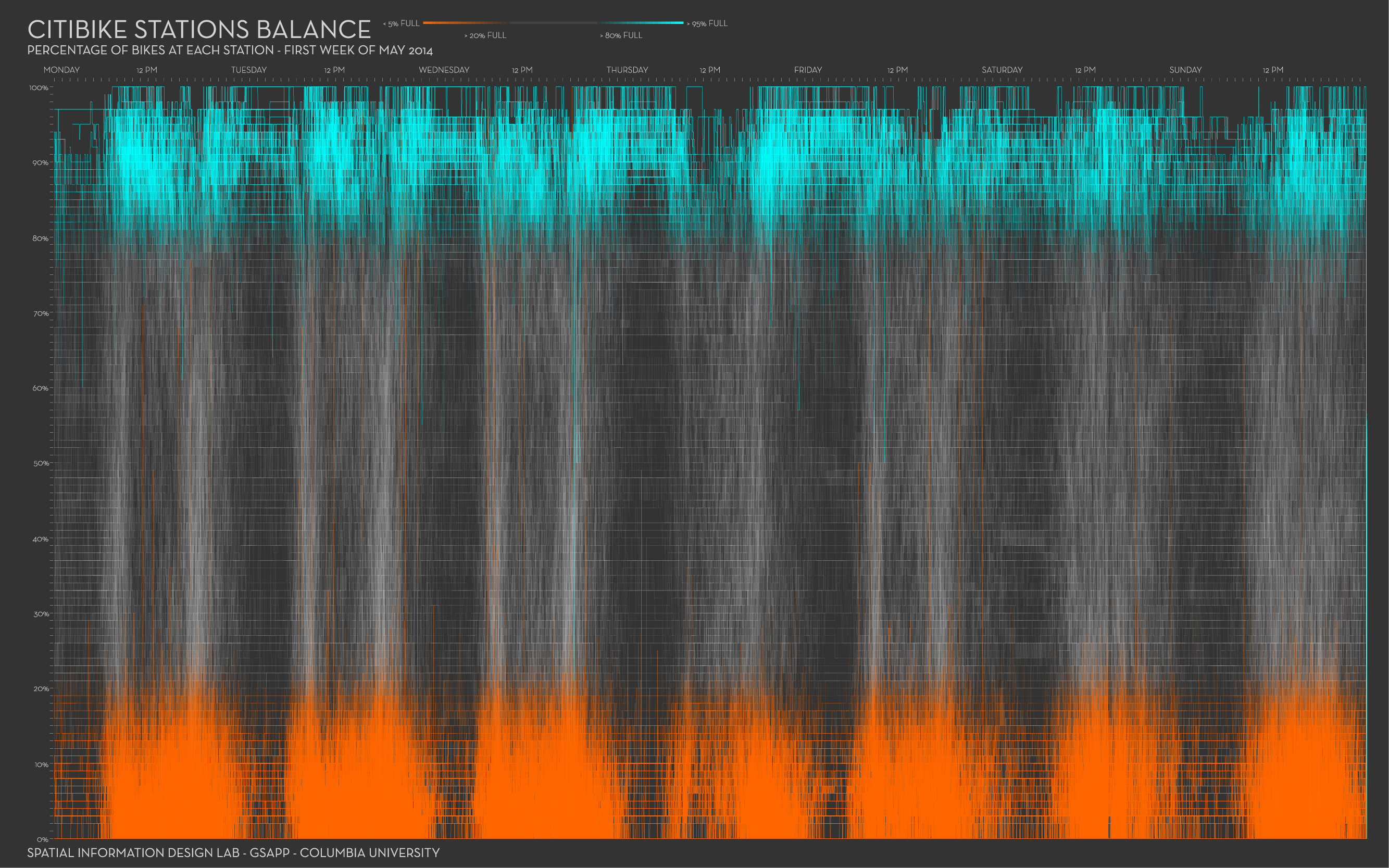
For the exercises below and similar to the further exercises for vega-lite, we will use the New York City citibike data available from https://www.citibikenyc.com/system-data. Some great visuals by Juan Francisco Saldarriaga can inspire you.

We made a (small) part of the data available here. It concerns trip data from November 2011, where the trip started or ended in station nr 336. The fields in each record (with example data) look like this:

{
  "tripduration": 1217,
  "starttime": "2019-11-01 06:03:28.5390",
  "stoptime": "2019-11-01 06:23:45.9810",
  "startstation_id": 3236,
  "startstation_name": "W 42 St & Dyer Ave",
  "startstation_latitude": 40.75898481399634,
  "startstation_longitude": -73.99379968643188,
  "endstation_id": 336,
  "endstation_name": "Sullivan St & Washington Sq",
  "endstation_latitude": 40.73047747,
  "endstation_longitude": -73.99906065,
  "bikeid": 41025,
  "usertype": "Subscriber",
  "birthyear": 1964,
  "gender": 1
}

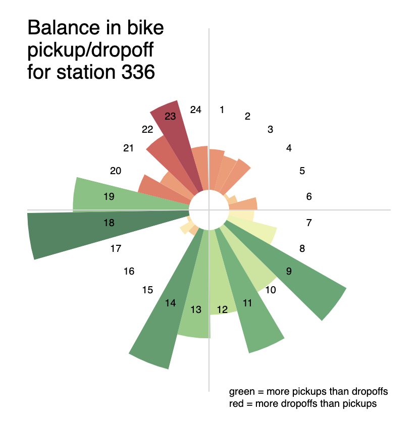
Exercise - Make a plot similar to the Citibike Station Dial shown here for station 336.

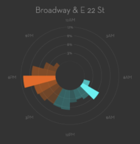
A possible output made with vega: