Branch Detection Benchmark

This notebook compares several clustering algorithms on their ability to detect branches in a dataset’s manifold that do not contain local density maxima. Our synthetic dataset contains several n-point star-shaped clusters and some uniform random noise. The stars have a density maximum in their centre, and the density decreases along their arms. A grid search is used to find the algorithms’ optimal parameter values, before their Adjusted Rand Index is used to compare their performance.

%load_ext autoreload
%autoreload 2

import time
import numpy as np
import pandas as pd
import matplotlib.pyplot as plt

from tqdm import tqdm
from itertools import product
from collections import defaultdict

from scipy import linalg
from sklearn.utils import shuffle
from sklearn.metrics.cluster import adjusted_rand_score

from lib.cdc import CDC
from sklearn.cluster import KMeans, AgglomerativeClustering, SpectralClustering
from fast_hbcc import HBCC, BoundaryClusterDetector
from fast_hdbscan import HDBSCAN, BranchDetector

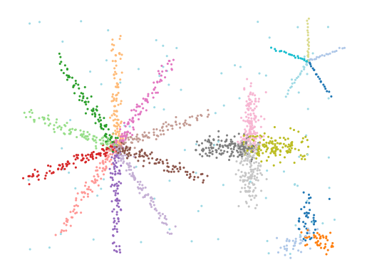
Datasets

The functions below make our benchmark dataset of 4 stars with varying densities and arms. The plot shows the ground-truth labels we will use to compute ARI scores.

def make_star(
    num_dimensions=2,
    num_branches=3,
    points_per_branch=100,
    branch_length=2,
    noise_scale=0.02,
):
    """Creates a n-star in d dimensions."""

    def rotation(axis=[0, 0, 1], theta=0):
        return linalg.expm(np.cross(np.eye(3), axis / linalg.norm(axis) * theta))

    def rotate(X, axis=[0, 0, 1], theta=0):
        M = rotation(axis=axis, theta=theta)
        data = np.hstack((X, np.zeros((X.shape[0], 1), dtype=X.dtype)))
        return (M @ data.T).T[:, :2]

    max_exp = np.log(branch_length)
    branch = np.zeros((points_per_branch, 2))
    branch[:, 0] = np.exp(np.linspace(0, max_exp, points_per_branch)) - 1
    branches = np.concatenate(
        [
            rotate(branch, theta=theta)
            for theta in np.linspace(0, 2 * np.pi, num_branches, endpoint=False)
            + np.pi / 2
        ]
    )
    X = np.column_stack((branches, np.zeros((branches.shape[0], num_dimensions - 2))))
    X += np.random.normal(
        scale=np.sqrt(1 / num_dimensions) * noise_scale,
        size=X.shape,
    )
    y = np.repeat(np.arange(num_branches), points_per_branch)
    return X, y


def make_stars_dataset(size_factor=1, num_dimensions=2):
    num_branches = [3, 10, 4, 5]
    branch_lengths = [1.8, 3.5, 2.3, 2]
    points_per_branch = [40, 100, 150, 20]
    noise_scales = [0.2, 0.1, 0.2, 0.02]
    origins = np.array(
        [
            [7, 1],
            [2, 3],
            [5.5, 3],
            [7, 5],
        ]
    )

    # Make individual starts
    Xs, ys = zip(
        *[
            make_star(
                num_dimensions=num_dimensions,
                num_branches=nb,
                branch_length=l,
                points_per_branch=int(np * size_factor),
                noise_scale=s,
            )
            for l, np, nb, s in zip(
                branch_lengths, points_per_branch, num_branches, noise_scales
            )
        ]
    )

    # Concatenate to one dataset
    X = np.concatenate(
        [
            x + np.concatenate((o, np.zeros(num_dimensions - 2)))
            for x, o in zip(Xs, origins)
        ]
    )
    y = np.concatenate(
        [y + nb for y, nb in zip(ys, [0] + np.cumsum(num_branches).tolist())]
    )

    # Add uniform noise points
    num_noise_points = X.shape[0] // 20
    noise_points = np.random.uniform(
        low=X.min(axis=0), high=X.max(axis=0), size=(num_noise_points, num_dimensions)
    )
    noise_labels = np.repeat(-1, num_noise_points)
    X = np.concatenate((X, noise_points))
    y = np.concatenate((y, noise_labels))

    # Shuffle the data
    return shuffle(X, y)

X, y = make_stars_dataset()
plot_kwargs = dict(s=5, cmap="tab20", vmin=0, vmax=19, edgecolors="k", linewidths=0)
plt.scatter(*X.T, c=y % 20, **plot_kwargs)
plt.axis("off")
plt.show()

Parameter Sweep

A parameter grid-search is used to find the optimal parameters for each algorithm. This ensures we are comparing the algorithms on their best performance. Searching all parameter combinations for all algorithms creates a too large search space. Instead we chose to keep some values at their defaults. We tried to mimic realistic use of the algorithms when selecting which parameters to keep at their default!

algorithms = dict(
    kmeans=KMeans,
    hdbscan=HDBSCAN,
    hbcc=HBCC,
    slink=AgglomerativeClustering,
    spectral=SpectralClustering,
    cdc=CDC,
)
post_processors = dict(
    flasc=BranchDetector,
    sbcc=BoundaryClusterDetector,
)
static_params = defaultdict(
    dict,
    slink=dict(linkage="single"),
    spectral=dict(assign_labels="cluster_qr"),
    flasc=dict(propagate_labels=True)
)

n_hops = [2, 3, 4, 5]
n_clusters = np.round(np.linspace(4, 25, 6)).astype(np.int32)
n_neighbors = np.round(np.linspace(2, 20, 6)).astype(np.int32)
min_cluster_sizes = np.unique(
    np.round(np.exp(np.linspace(np.log(25), np.log(60), 10)))
).astype(np.int32)
selection_methods = ["eom", "leaf"]
hop_types = ["manifold", "metric"]


dynamic_params = defaultdict(
    dict,
    kmeans=dict(n_clusters=n_clusters),
    slink=dict(n_clusters=n_clusters),
    spectral=dict(n_clusters=n_clusters),
    cdc=dict(k=n_neighbors, ratio=np.linspace(0.5, 0.95, 2).round(4)),
    hdbscan=dict(
        min_samples=n_neighbors,
        min_cluster_size=min_cluster_sizes,
        cluster_selection_method=selection_methods,
    ),
    hbcc=dict(
        num_hops=n_hops,
        hop_type=hop_types,
        min_samples=n_neighbors,
        min_cluster_size=min_cluster_sizes,
        cluster_selection_method=selection_methods,
    ),
    sbcc=dict(num_hops=n_hops, hop_type=hop_types),
)

all_params = {name for params in dynamic_params.values() for name in params.keys()}

# compile all code paths for timing to be true.
_ = HBCC().fit(X)
_ = HBCC(cluster_selection_method='leaf').fit(X)
_ = HBCC(hop_type='metric').fit(X)
eomc = HDBSCAN().fit(X)
leafc = HDBSCAN(cluster_selection_method='leaf').fit(X)
_ = BoundaryClusterDetector().fit(eomc)
_ = BoundaryClusterDetector().fit(leafc)
_ = BranchDetector().fit(eomc)
_ = BranchDetector().fit(leafc)

# Create output structure
results = {
    "repeat": [],
    "alg": [],
    "ari": [],
    "time": [],
    "labels": [],
    **{name: [] for name in all_params},
}


def process_algorithm(X, alg_name, alg_class, **base_kwargs):
    kwargs = static_params[alg_name]
    dynamic_ranges = dynamic_params[alg_name]
    for values in product(*dynamic_ranges.values()):
        params = {param: value for param, value in zip(dynamic_ranges.keys(), values)}
        complete_params = {**base_kwargs, **params}
        start = time.perf_counter()
        cc = alg_class(**kwargs, **params)
        labels = cc.fit_predict(X)
        end = time.perf_counter()

        results["repeat"].append(r)
        results["alg"].append(alg_name)
        results["ari"].append(adjusted_rand_score(y, labels))
        results["time"].append(end - start)
        results["labels"].append(labels)

        for name in all_params:
            results[name].append(complete_params.get(name, np.nan))

        if alg_name == "hdbscan":
            for post_name, detector_class in post_processors.items():
                process_algorithm(cc, post_name, detector_class, **params)


for r in tqdm(range(5)):
    # Generate dataset
    X, y = make_stars_dataset()
    np.save(f"data/generated/star_parameter_sweep_X_{r}", X)
    np.save(f"data/generated/star_parameter_sweep_y_{r}", y)

    # Run the parameter sweep
    for alg_name, alg_class in algorithms.items():
        process_algorithm(X, alg_name, alg_class)

# Store the results!
result_df = pd.DataFrame.from_dict(results)
result_df.to_parquet("data/generated/star_parameter_sweep_results.parquet")

100%|██████████| 5/5 [09:25<00:00, 113.02s/it]

Results

Now, we can compare the clusters found by each algorithm with their optimal parameter values. NaN values indicate parameters that are not used by that particular algorithm.

result_df = pd.read_parquet("data/generated/star_parameter_sweep_results.parquet")
best_cases = result_df.loc[result_df.groupby(['alg']).apply(lambda x: x.index[np.argmax(x.ari)]).values]
best_cases.drop(columns=['labels'])

C:\Users\jelme\AppData\Local\Temp\ipykernel_19884\2953733996.py:2: DeprecationWarning: DataFrameGroupBy.apply operated on the grouping columns. This behavior is deprecated, and in a future version of pandas the grouping columns will be excluded from the operation. Either pass `include_groups=False` to exclude the groupings or explicitly select the grouping columns after groupby to silence this warning.
  best_cases = result_df.loc[result_df.groupby(['alg']).apply(lambda x: x.index[np.argmax(x.ari)]).values]

	repeat	alg	ari	time	hop_type	n_clusters	num_hops	cluster_selection_method	ratio	min_samples	min_cluster_size	k
4370	1	cdc	0.279661	0.964522	None	NaN	NaN	None	0.5	NaN	NaN	6.0
207	0	flasc	0.621272	0.004027	None	NaN	NaN	eom	NaN	6.0	25.0	NaN
5948	2	hbcc	0.431407	0.005967	metric	NaN	3.0	eom	NaN	2.0	28.0	NaN
8766	4	hdbscan	0.233489	0.004590	None	NaN	NaN	eom	NaN	2.0	25.0	NaN
8764	4	kmeans	0.362905	0.003664	None	21.0	NaN	None	NaN	NaN	NaN	NaN
7010	3	sbcc	0.583484	0.028694	manifold	NaN	3.0	leaf	NaN	9.0	28.0	NaN
4361	1	slink	0.151713	0.010276	None	25.0	NaN	None	NaN	NaN	NaN	NaN
4365	1	spectral	0.347316	0.174356	None	17.0	NaN	None	NaN	NaN	NaN	NaN

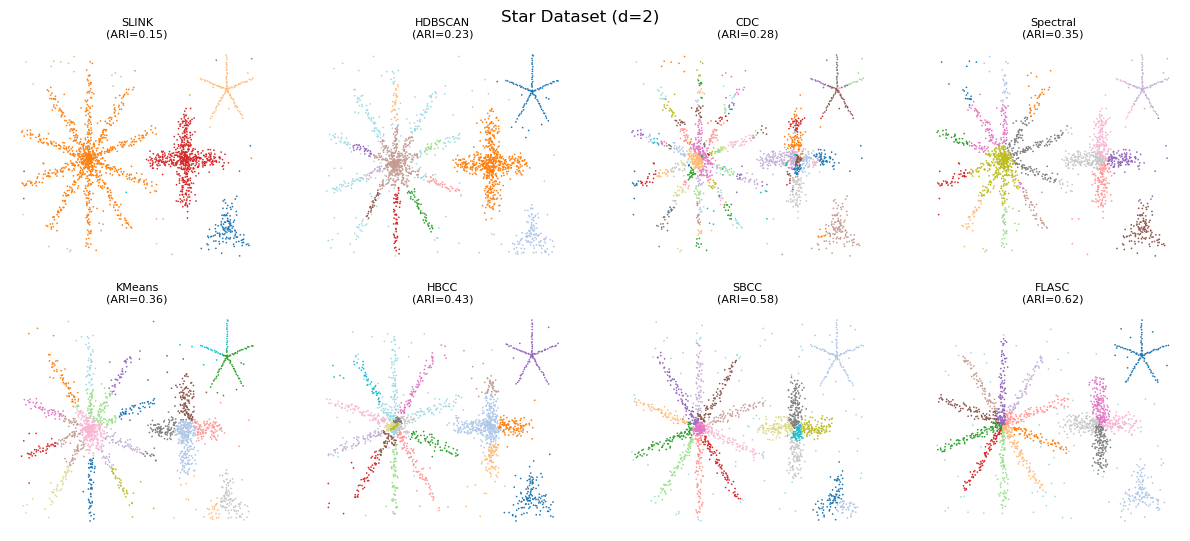
Detected Clusters

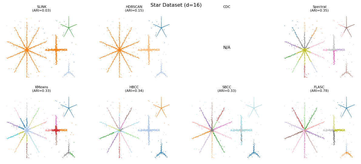
This case shows the algorithms on 2D data, with optimal parameters found on 2D data. As expected, the distance- and density-based algorithms have the lowest ARI values, mostly separating the stars as clusters and not finding the branches. CDC sometimes finds branches as a single cluster but more often finds multiple smaller clusters where we expect a single branch. The main problem it faces is that it does not sufficiently limit the connectivity that is allowed to exist between points, leading to spurious connections linking clusters that should remain separate. k-Means and spectral clustering sometimes find branches as clusters but also create clusters that combine multiple branches into one label. HBCC and SBCC (SBCC is HBCC on HDBSCAN clusters) are quite good in finding the branches, but also give the centres a label. FLASC has the highest ARI scores, but also fails to find branches in smaller stars. Performance of HBCC, SBCC, and FLASC could be improved by separating the min cluster size and min branch size parameter values.

plt.figure(figsize=(12, 6))
algs = ["slink", "hdbscan", "cdc", "spectral", "kmeans", "hbcc", "sbcc", "flasc"]
names = ['SLINK', 'HDBSCAN', 'CDC', 'Spectral', 'KMeans', "HBCC", "SBCC", 'FLASC']
cnt = 1
for alg, alg_name in zip(algs, names):
    plt.subplot(2, 4, cnt)
    plt.xticks([])
    plt.yticks([])
    plt.gca().spines["top"].set_visible(False)
    plt.gca().spines["right"].set_visible(False)
    plt.gca().spines["bottom"].set_visible(False)
    plt.gca().spines["left"].set_visible(False)
    cnt += 1
    row = best_cases.query("alg == @alg")
    if row.shape[0] == 0:
        plt.text(0.5, 0.5, "N/A", fontsize=10, ha="center", va="center")
        plt.title(f"{alg_name}\n", fontsize=8)
        continue
    plt.title(f"{alg_name}\n(ARI={row.ari.iloc[0]:.2f})", fontsize=8)

    plt.scatter(
        *np.load(
            f"data/generated/star_parameter_sweep_X_{row.repeat.iloc[0]}.npy"
        )[:, :2].T,
        s=1.5,
        c=row.labels.iloc[0] % 20,
        cmap="tab20",
        vmin=0,
        vmax=19,
        edgecolors="none",
        linewidths=0,
    )
plt.subplots_adjust(left=0.025, right=1, top=0.92)
plt.suptitle(f"Star Dataset (d=2)", fontsize=12)
plt.show()

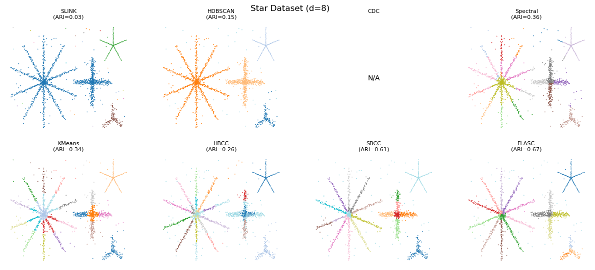
Higher Dimensions Data

Just to check, we now run the algorithms on 8D and 16D data with their optimal parameters found on 2D data. Only the noise is present in the higher dimensions. Performance increases for FLASC. HBCC and SBCC seem to have trouble with the additional dimensions. It appears the boundary coefficient needs tuning for these cases.

for d in [8, 16]:
    X, y = make_stars_dataset(num_dimensions=d)

    plt.figure(figsize=(12, 6))
    cnt = 1
    for alg, alg_name in zip(algs, names):
        plt.subplot(2, 4, cnt)
        plt.xticks([])
        plt.yticks([])
        plt.gca().spines["top"].set_visible(False)
        plt.gca().spines["right"].set_visible(False)
        plt.gca().spines["bottom"].set_visible(False)
        plt.gca().spines["left"].set_visible(False)
        cnt += 1
        if alg == "cdc":
            plt.text(0.5, 0.5, "N/A", fontsize=10, ha="center", va="center")
            plt.title(f"{alg_name}\n", fontsize=8)
            continue

        row = best_cases.query("alg == @alg")
        kwargs = static_params[alg]
        params = {k: row[k].iloc[0] for k in dynamic_params[alg].keys()}
        params = {
            k: int(v) if isinstance(v, np.floating) else str(v)
            for k, v in params.items()
        }
        if alg in ["sbcc", "flasc"]:
            hkwargs = static_params["hdbscan"]
            hparams = {k: row[k].iloc[0] for k in dynamic_params["hdbscan"].keys()}
            hparams = {
                k: int(v) if isinstance(v, np.floating) else str(v)
                for k, v in hparams.items()
            }
            cc = HDBSCAN(**hkwargs, **hparams).fit(X)
            dd = post_processors[alg](**kwargs).fit(cc)
            labels = dd.fit_predict(cc)
        else:
            labels = algorithms[alg](**kwargs, **params).fit_predict(X)
        ari = adjusted_rand_score(y, labels)
        plt.title(f"{alg_name}\n(ARI={ari:.2f})", fontsize=8)

        plt.scatter(
            *X[:, :2].T,
            s=1.5,
            c=labels % 20,
            cmap="tab20",
            vmin=0,
            vmax=19,
            edgecolors="none",
            linewidths=0,
        )
    plt.subplots_adjust(left=0.025, right=1, top=0.92)
    plt.suptitle(f"Star Dataset (d={X.shape[1]})", fontsize=12)
    plt.show()

Parameter Sensitivity

Now we explore the algorithm’s parameter sensitivity using average ARI and compute time over the 5 repeated runs.

avg_df = result_df.query("repeat == 0")[["alg", *all_params]].copy()
avg_df["ari"] = np.mean(
    np.stack([result_df.query("repeat == @i").ari.values for i in range(5)]),
    axis=0,
)
avg_df["time"] = np.mean(
    np.stack([result_df.query("repeat == @i").time.values for i in range(5)]),
    axis=0,
)

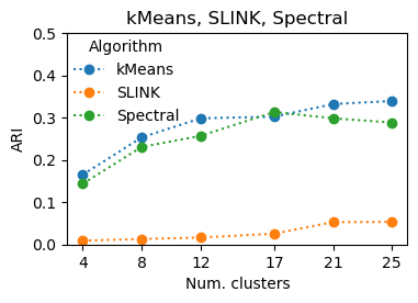
kMeans, SLINK, Spectral

These algorithms require the number of clusters as input. The true number is 23 and performance peaks around there for these algorithms.

plt.figure(figsize=(4, 2.5))
avg_df[~np.isnan(avg_df.n_clusters)].pivot(
    index="n_clusters", columns="alg", values="ari"
).plot(xlabel="Num. clusters", ylabel="ARI", linestyle=":", marker="o", ax=plt.gca())
plt.legend(
    ["kMeans", "SLINK", "Spectral"], title="Algorithm", borderaxespad=0, frameon=False
)
plt.xticks(n_clusters)
plt.ylim(0, 0.5)
plt.title("kMeans, SLINK, Spectral")
plt.show()

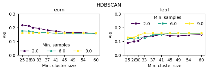
HDBSCAN

HDBSCAN performs best with low min_samples and min_cluster_size because that is when it is most sensitive to small density peaks—the only way in which it can detect clusters that do not have a reliable density peak.

import seaborn as sns

plt.figure(figsize=(8, 2))
for i, strat in enumerate(["eom", "leaf"]):
    plt.subplot(1, 2, i + 1)
    sns.lineplot(
        avg_df.query(
            "alg == 'hdbscan' and "
            "min_samples < 10 and "
            "cluster_selection_method==@strat"
        ).rename(
            columns=dict(
                min_samples="Min. samples", cluster_selection_method="Selection"
            )
        ),
        marker="o",
        x="min_cluster_size",
        y="ari",
        hue="Min. samples",
        palette="viridis",
    )
    plt.legend(ncols=3, borderaxespad=0, frameon=False, title='Min. samples')
    plt.xticks(min_cluster_sizes)
    plt.xlabel("Min. cluster size")
    plt.ylabel("ARI")
    plt.ylim(0, 0.3)
    plt.title(strat)
plt.suptitle("HDBSCAN")
plt.subplots_adjust(wspace=0.3, top=0.8)
plt.show()

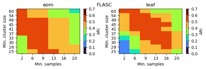
FLASC (BranchDetector)

FLASC performs well on a larger range of parameter values. It needs a relatively low min_samples to avoid min_samples-nearest neighbors connecting branches at high eccentricity values. The minimum cluster size needs to be smaller than the true number of points in the smallest branch. Too small values tend to produce spurious branches. In this case, values between 25 and 49 work well. The leaf selection strategy is more sensitive to min_samples, as it influences the number of leafs.

import matplotlib as mpl
from matplotlib.colors import BoundaryNorm

bounds = np.linspace(0, 0.7, 8)
cmap = mpl.colormaps["turbo"]
norm = BoundaryNorm(bounds, cmap.N)


plt.figure(figsize=(8, 2))
for i, strat in enumerate(["eom", "leaf"]):
    plt.subplot(1, 2, i + 1)
    flasc2d = avg_df.query("alg=='flasc' and cluster_selection_method==@strat")
    plt.imshow(
        flasc2d.pivot(index="min_cluster_size", columns="min_samples", values="ari"),
        origin="lower",
        aspect="auto",
        cmap=cmap,
        norm=norm,
    )
    plt.xticks(range(len(n_neighbors)))
    plt.yticks(range(len(min_cluster_sizes)))
    plt.gca().set_xticklabels([f"{int(x)}" for x in n_neighbors])
    plt.gca().set_yticklabels([f"{int(x)}" for x in min_cluster_sizes])

    plt.xlabel("Min. samples")
    plt.ylabel("Min. cluster size")
    plt.colorbar(label="ARI")
    plt.title(strat)
plt.subplots_adjust(wspace=0.3)
plt.suptitle("FLASC")
plt.show()

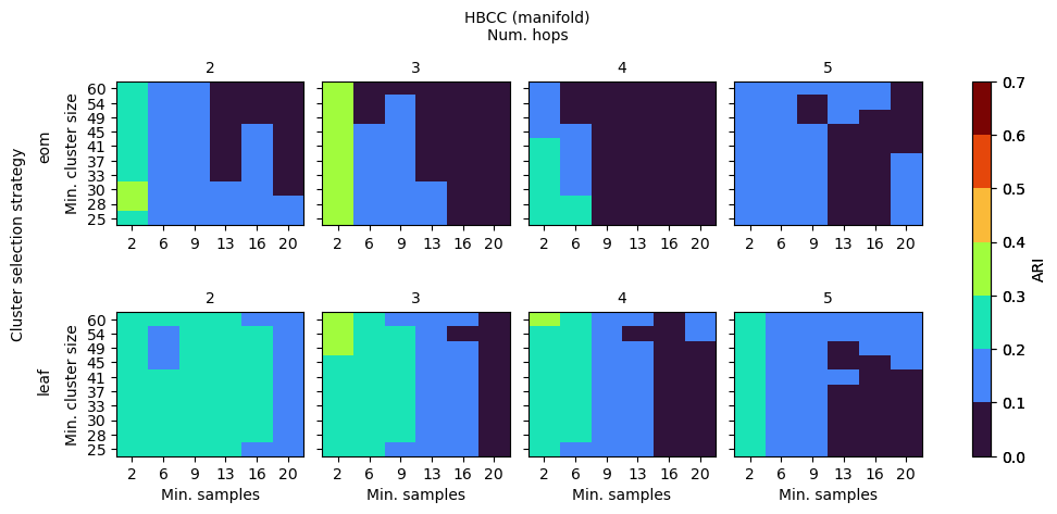
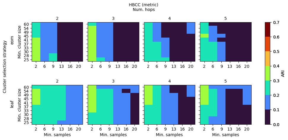
HBCC

HBCC’s parameters influence both the shape of the coreness profile as well as the way in which clusters are extracted from the profile. Generally, for this data set, low values for num_hops and min_samples are needed for there to be coreness maxima in the branches. When those maxima exist, min_cluster_size can vary between 25 to 60, indicating a lower sensitivity.

for hoptype in hop_types:
    plt.figure(figsize=(12, 5))
    for j, strat in enumerate(["eom", "leaf"]):
        hbcc2d = avg_df.query("alg=='hbcc' and cluster_selection_method==@strat and hop_type==@hoptype")
        for i, bs in enumerate(n_hops):
            plt.subplot(2, 5, j * 5 + i + 1)
            plt.imshow(
                hbcc2d.query("num_hops == @bs").pivot(
                    index="min_cluster_size", columns="min_samples", values="ari"
                ),
                origin="lower",
                aspect="auto",
                cmap=cmap,
                norm=norm,
            )
            plt.xticks(range(len(n_neighbors)))
            plt.yticks(range(len(min_cluster_sizes)))
            plt.gca().set_xticklabels([f"{int(x)}" for x in n_neighbors])
            plt.gca().set_yticklabels([f"{int(x)}" for x in min_cluster_sizes])

            if j == 1:
                plt.xlabel("Min. samples")
            if i == 0:
                plt.ylabel("Min. cluster size")
            else:
                plt.gca().set_yticklabels(["" for _ in min_cluster_sizes])
            plt.title(f"{bs}", fontsize=10)

        ax = plt.subplot(1, 6, 6)
        plt.colorbar(ax=ax, aspect=20, pad=0, fraction=1, label="ARI")
        plt.axis("off")
        plt.text(
            0.07,
            0.68 if j == 0 else 0.25,
            strat,
            fontsize=10,
            ha="center",
            va="center",
            rotation=90,
            transform=plt.gcf().transFigure,
        )
    plt.text(
        0.44,
        0.9,
        f"HBCC ({hoptype})\nNum. hops",
        fontsize=10,
        ha="center",
        va="center",
        transform=plt.gcf().transFigure,
    )
    plt.text(
        0.05,
        0.5,
        "Cluster selection strategy",
        fontsize=10,
        ha="center",
        va="center",
        rotation=90,
        transform=plt.gcf().transFigure,
    )
    plt.subplots_adjust(top=0.8, hspace=0.6, wspace=0.1)
    plt.show()

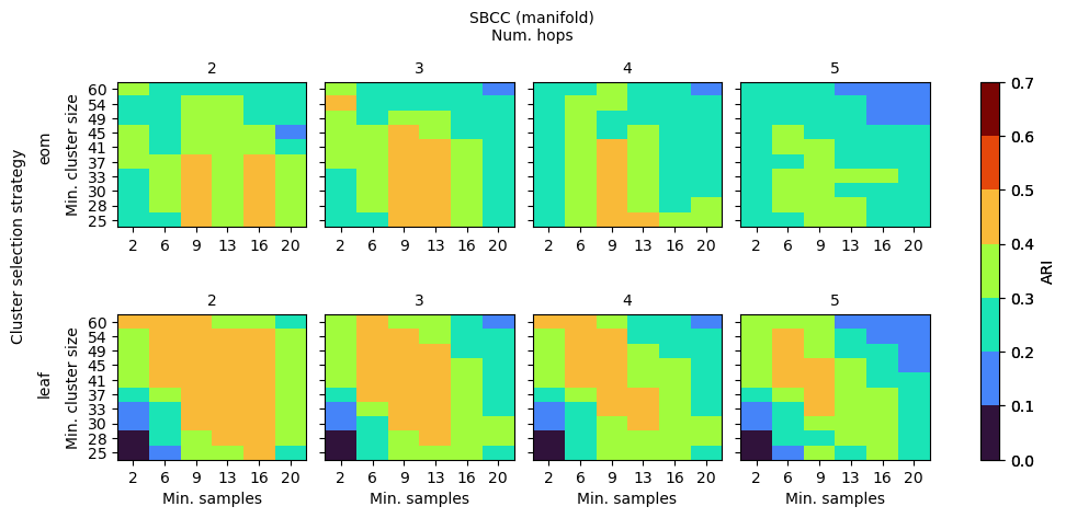
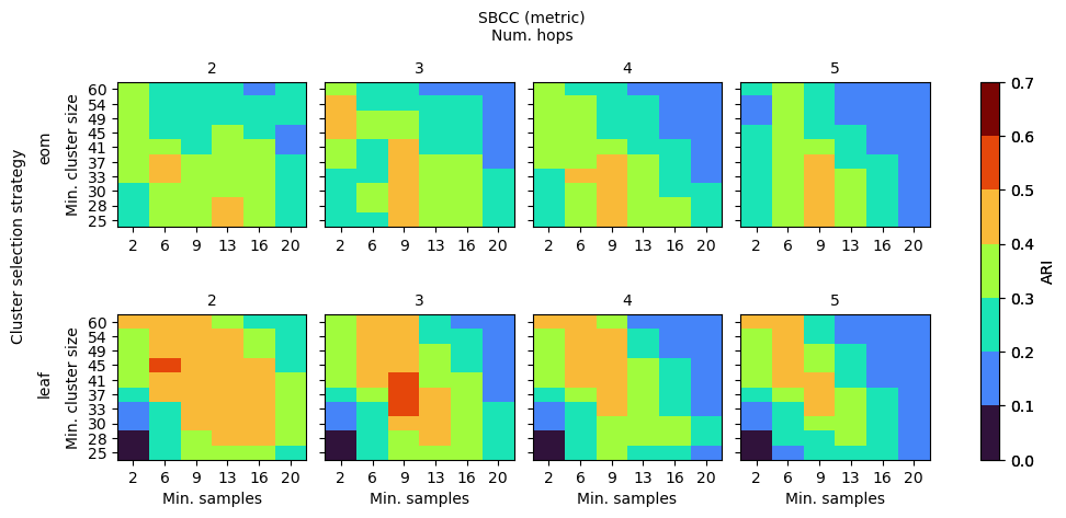
SBCC (BoundaryClusterDetector)

SBCC’s parameters behave a bit differently. Noise is already dealt with by HDBSCAN, so slightly larger num_hops and min_samples create a smoother coreness profile to extract the clusters from. Separating the cluster selection strategy between the HDBSCAN and HBCC stages would provide a larger range of good performing parameter values, as HDBCC works best with leaf, while HDBSCAN is most stable with eom.

for hoptype in hop_types:
    plt.figure(figsize=(12, 5))
    for j, strat in enumerate(["eom", "leaf"]):
        sbcc2d = avg_df.query("alg=='sbcc' and cluster_selection_method==@strat and hop_type==@hoptype")
        for i, bs in enumerate(n_hops):
            plt.subplot(2, 5, j * 5 + i + 1)
            plt.imshow(
                sbcc2d.query("num_hops == @bs").pivot(
                    index="min_cluster_size", columns="min_samples", values="ari"
                ),
                origin="lower",
                aspect="auto",
                cmap=cmap,
                norm=norm,
            )
            plt.xticks(range(len(n_neighbors)))
            plt.yticks(range(len(min_cluster_sizes)))
            plt.gca().set_xticklabels([f"{int(x)}" for x in n_neighbors])
            plt.gca().set_yticklabels([f"{int(x)}" for x in min_cluster_sizes])

            if j == 1:
                plt.xlabel("Min. samples")
            if i == 0:
                plt.ylabel("Min. cluster size")
            else:
                plt.gca().set_yticklabels(["" for _ in min_cluster_sizes])
            plt.title(f"{bs}", fontsize=10)

        ax = plt.subplot(1, 6, 6)
        plt.colorbar(ax=ax, aspect=20, pad=0, fraction=1, label="ARI")
        plt.axis("off")
        plt.text(
            0.07,
            0.68 if j == 0 else 0.25,
            strat,
            fontsize=10,
            ha="center",
            va="center",
            rotation=90,
            transform=plt.gcf().transFigure,
        )
    plt.text(
        0.44,
        0.9,
        f"SBCC ({hoptype})\nNum. hops",
        fontsize=10,
        ha="center",
        va="center",
        transform=plt.gcf().transFigure,
    )
    plt.text(
        0.05,
        0.5,
        "Cluster selection strategy",
        fontsize=10,
        ha="center",
        va="center",
        rotation=90,
        transform=plt.gcf().transFigure,
    )
    plt.subplots_adjust(top=0.8, hspace=0.6, wspace=0.1)
    plt.show()

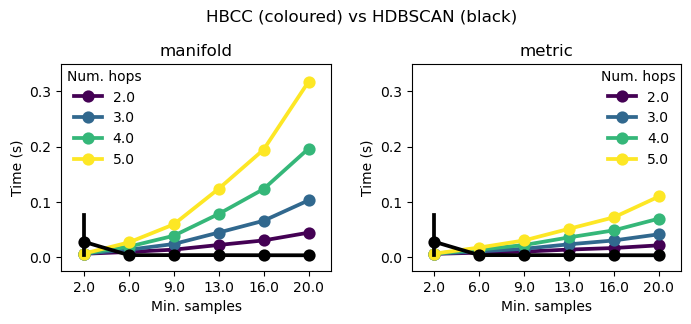
HBCC Compute Time

Compute cost for the boundary coefficient increases with the product of num_hops and min_samples because num_hop controls the depth of a Dijkstra’s shortest path algorithm and min_samples controls the number of edges each point has. Furthermore, computing the boundary coefficient relies on a sparse matrix multiplication, which scales by the number of edges in the expanded graph.

In the figure below, HDBSCAN’s time is shown in black. It appears one code path for HDBSCAN was not pre-compiled, leading to the larger uncertainty at min_samples=2.

plt.figure(figsize=(8, 3))
for i, hoptype in enumerate(hop_types):
    plt.subplot(1, 2, i+1)
    sns.pointplot(
        avg_df.query("alg=='hbcc' and cluster_selection_method==@strat and hop_type==@hoptype"),
        x="min_samples",
        y="time",
        hue="num_hops",
        marker="o",
        palette="viridis",
        legend=True,
    )
    sns.pointplot(
        avg_df.query("alg == 'hdbscan'"),
        x="min_samples",
        y="time",
        color="k",
        legend=False,
    )
    plt.legend(title="Num. hops", borderaxespad=0, frameon=False)
    plt.xlabel("Min. samples")
    plt.ylabel("Time (s)")
    plt.ylim([-0.025, 0.35])
    plt.title(hoptype)
plt.suptitle("HBCC (coloured) vs HDBSCAN (black)")
plt.subplots_adjust(wspace=0.3, top=0.8)
plt.show()