Manifold Modelling with Minimum Spanning Trees

Dimensionality reduction (DR) algorithms typically assume the data they are given is uniformly sampled from some underlying manifold. When this is not the case, and there are observation-gaps along the manifold, these algorithms may fail to detect a single connected entity. This repository presents two manifold approximation approaches based on minimum spanning trees (MST) for non-uniform sampled data.

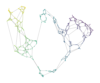
Noisy Minimum Spanning Tree Union

The noisy minimum spanning tree union (n-MST) is inspired by Pathfinder networks that, with a specific parameter selection, yield the union set of all possible MSTs in a network (see, e.g., [1], [2]). We compute noisy MSTs to detect alternative connectivity at all distance scales for distances which may have few identically weighted connections.

We add Gaussian noise (mean=0) to every candidate edge. The noise parameter n is specified as a fraction of the points’ nearest neighbour distance and controls the Gaussian’s standard deviation. This formulation makes the noise scale with the data’s density to avoid adding more edges in dense regions than sparse regions, retaining a reasonably uniform manifold approximation graph.

import matplotlib.pyplot as plt
import matplotlib.collections as mc
from sklearn.datasets import make_swiss_roll
from multi_mst.noisy_mst import NoisyMST

X, t = make_swiss_roll(n_samples=2000, noise=0.5, hole=True)
projector = NoisyMST(num_trees=10, noise_fraction=1.0).fit(X)

# Draw the network
xs = projector.embedding_[:, 0]
ys = projector.embedding_[:, 1]
coo_matrix = projector.graph_.tocoo()
sources = coo_matrix.row
targets = coo_matrix.col

plt.figure(figsize=(4, 3))
plt.scatter(xs, ys, c=t, s=1, edgecolors="none", linewidth=0, cmap="viridis")
lc = mc.LineCollection(
    list(zip(zip(xs[sources], ys[sources]), zip(xs[targets], ys[targets]))),
    linewidth=0.2,
    zorder=-1,
    alpha=0.5,
    color="k",
)
ax = plt.gca()
ax.add_collection(lc)
ax.set_aspect("equal")
plt.subplots_adjust(0, 0, 1, 1)
plt.axis("off")
plt.show()

k-Nearest Minimum Spanning Tree

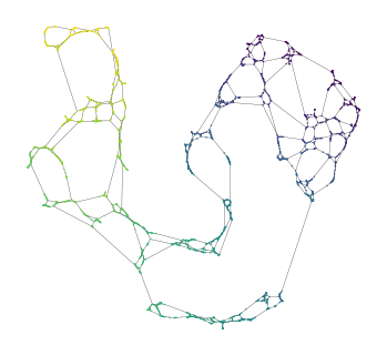
The k-nearest Minimum Spanning Tree (k-MST) generalises k-nearest neighbour networks (k-NN) for minimum spanning trees. It adds the k shortest edges between components. Since data points start as distinct components, all k-NN edges are included in the kMST.

To avoid creating shortcuts in the manifold, a distance threshold epsilon can be applied. The parameter is specified as a fraction of the shortest edge between components and provides an upper distance limit for the 2-to-k alternative edges.

import matplotlib.pyplot as plt
import matplotlib.collections as mc
from sklearn.datasets import make_swiss_roll
from multi_mst.k_mst import KMST

X, t = make_swiss_roll(n_samples=2000, noise=0.5, hole=True)
projector = KMST(num_neighbors=3, epsilon=2.0).fit(X)

# Draw the network
xs = projector.embedding_[:, 0]
ys = projector.embedding_[:, 1]
coo_matrix = projector.graph_.tocoo()
sources = coo_matrix.row
targets = coo_matrix.col

plt.figure(figsize=(4, 3))
plt.scatter(xs, ys, c=t, s=1, edgecolors="none", linewidth=0, cmap="viridis")
lc = mc.LineCollection(
    list(zip(zip(xs[sources], ys[sources]), zip(xs[targets], ys[targets]))),
    linewidth=0.2,
    zorder=-1,
    alpha=0.5,
    color="k",
)
ax = plt.gca()
ax.add_collection(lc)
ax.set_aspect("equal")
plt.subplots_adjust(0, 0, 1, 1)
plt.axis("off")
plt.show()

Approximate k-MST

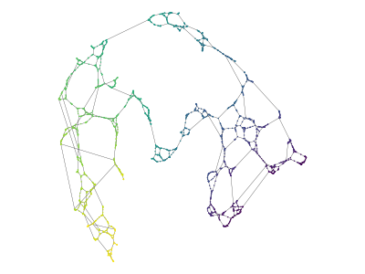
Computing k-MSTs using KDTrees can be expensive on some datasets. We provide a version of the algorithm based on Nearest Neighbour Descent for quicker approximations. We combined Boruvka’s algorithm with NNDescent to find neighbours that are not already connected in the MST being build.

import matplotlib.pyplot as plt
import matplotlib.collections as mc
from sklearn.datasets import make_swiss_roll
from multi_mst.k_mst_descent import KMSTDescent

X, t = make_swiss_roll(n_samples=2000, noise=0.5, hole=True)
projector = KMSTDescent(num_neighbors=3, epsilon=2.0).fit(X)

# Draw the network
xs = projector.embedding_[:, 0]
ys = projector.embedding_[:, 1]
coo_matrix = projector.graph_.tocoo()
sources = coo_matrix.row
targets = coo_matrix.col

plt.figure(figsize=(4, 3))
plt.scatter(xs, ys, c=t, s=1, edgecolors="none", linewidth=0, cmap="viridis")
lc = mc.LineCollection(
    list(zip(zip(xs[sources], ys[sources]), zip(xs[targets], ys[targets]))),
    linewidth=0.2,
    zorder=-1,
    alpha=0.5,
    color="k",
)
ax = plt.gca()
ax.add_collection(lc)
ax.set_aspect("equal")
plt.subplots_adjust(0, 0, 1, 1)
plt.axis("off")
plt.show()

Installation Instructions

The multi_mst package can be installed from pypi:

pip install multi_mst

Acknowledgements

Most code—including the numba KDTree, disjoint set and boruvka MST construction implementation—is adapted from fast_hdbscan. The NNDescent implementation is adapted from pynndescent.

License

multi_mst uses the same license as fast_hdbscan: BSD (2-clause). See the LICENSE file for details.