Beyond SQL
This post is part of the course material for the Software and Data Management course at UHasselt. The contents of this post is licensed as CC-BY: feel free to copy/remix/tweak/… it, but please credit your source.

For a particular year’s practicalities, see http://vda-lab.be/teaching
Table of contents
- Table of contents
- 1. Some issues with relational databases
- 2. Intermezzo: JSON
- 3. Key-value stores
- 4. Document-oriented databases
- 5. Graph databases
- 6. ArangoDB - a multi-model database
- 7. Using ArangoDB from R
1. Some issues with relational databases
Although relational databases have been used for multiple decades and are easy to get started with, they do have some shortcomings, particularly in the big data era that we’re in now.
1.1 Querying scalability: joins
Best practices in relational database design call for a normalised design (see in our previous post). This means that the different concepts in the data are separated out into tables, and can be joined together again in a query. Unfortunately, joins can be very expensive. For example, the Ensembl database (www.ensembl.org) is a fully normalised omics database, containing a total of 74 tables. For example, to get the exon positions for a given gene, one needs to run 3 joins.
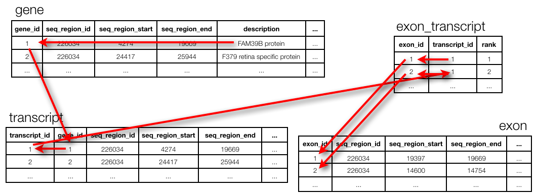
(Actually: note that this ends at seq_region and not at chromosome. To get to the chromosome actually requires two more joins but those are too complex to explain in the context of this session…)
The query to get the exon positions for FAM39B protein:
SELECT e.seq_region_start
FROM gene g, transcript t, exon_transcript et, exon e
WHERE g.description = 'FAM39B protein'
AND g.gene_id = t.gene_id
AND t.transcript_id = et.transcript_id
AND et.exon_id = e.exon_id;
1.2 Writing scalability
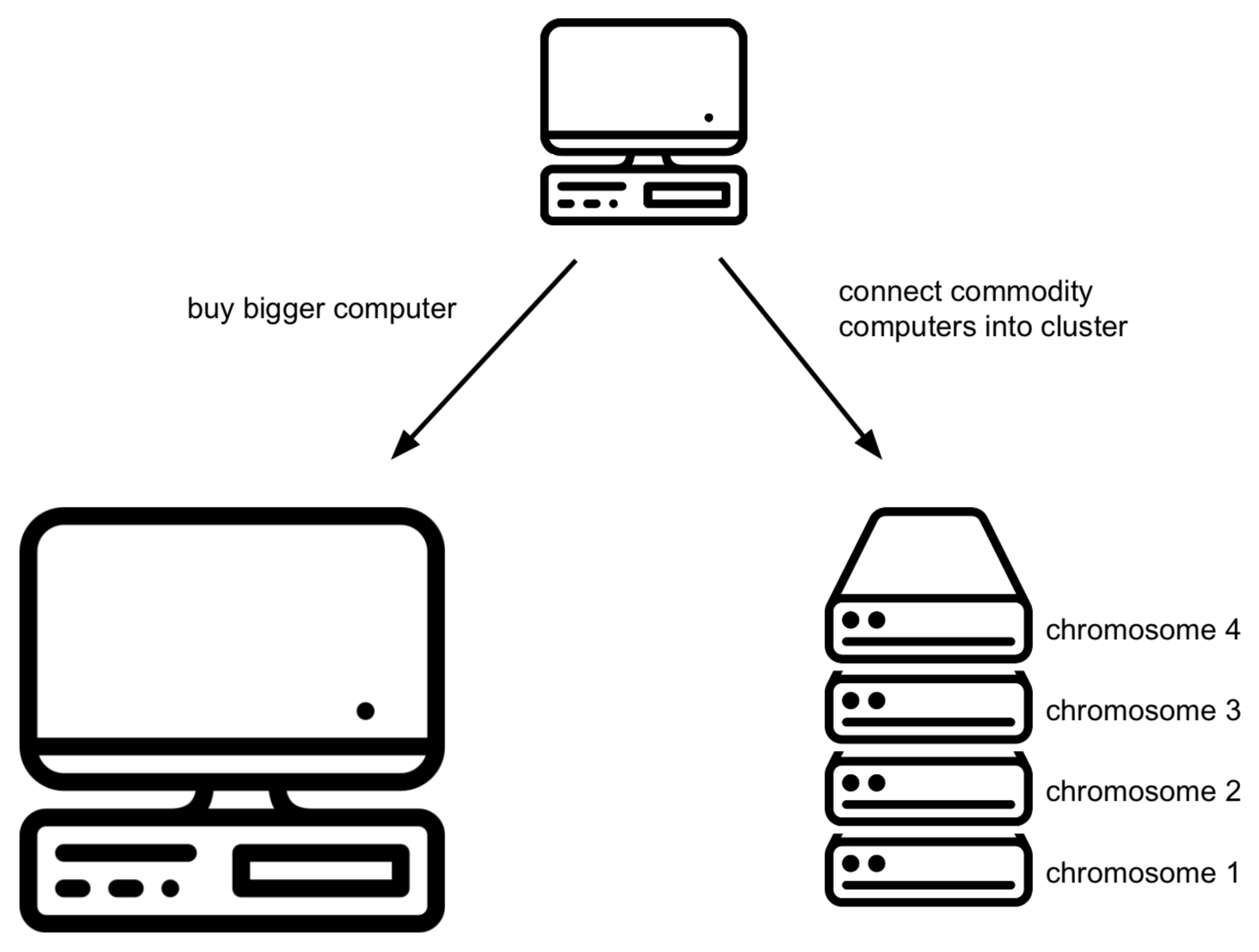
Suppose that you begin to store genomic mutations in a mysql database. All goes well, until you notice that the database becomes too large for the computer you are running mysql on. There are different solutions for this:
- Buy a bigger computer (= vertical scaling) which will typically be much more expensive
- Shard your data across different databases on different computers (= horizontal scaling): data for chromosome 1 is stored in a mysql database on computer 1, chromosome 2 is stored in a mysql database on computer 2, etc. Unfortunately, this does mean that in your application code (i.e. when you’re trying to access this data from R or python), you need to know what computer to connect to. It gets worse if you later notice that one of these other servers becomes the bottleneck. Then you’d have to get additional computers and e.g. store the first 10% of chromosome 1 on computer 1, the next 10% on computer 2, etc. Again: this makes it very complicated in your R and/or python scripts as you have to know what is stored where.
1.3 Relational data
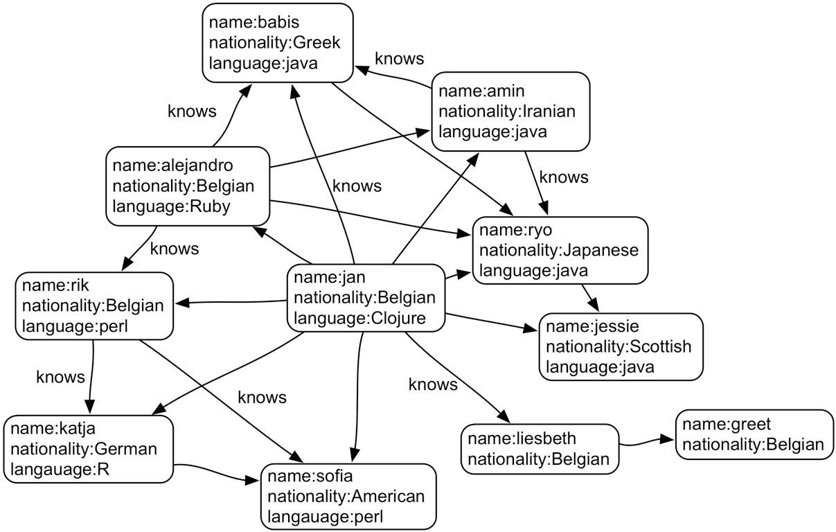
Imagine you have a social graph and the data is stored in a relational database. People have names, and know other people. Every “know” is reciprocal (so if I know you then you know me too).
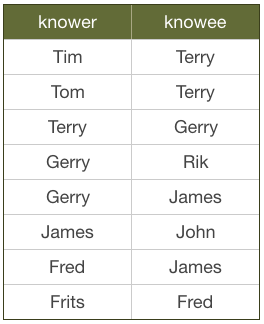
Let’s see what it means to follow relationships in a RDBMS. What would this look like if we were searching for friends of James?
SELECT knowee FROM friends
WHERE knower IN (
  SELECT knowee FROM friends
  WHERE knower = 'James'
  )
UNION
SELECT knower FROM friends
WHERE knowee IN (
  SELECT knower FROM friends
  WHERE knowee = 'James'
  );
Quite verbose. What if we’d want to go one level deeper: all friends of friends of James?
SELECT knowee FROM friends
WHERE knower IN (
  SELECT knowee FROM friends
  WHERE knower IN (
    SELECT knowee FROM friends
    WHERE knower = 'James'
    )
  UNION
  SELECT knower FROM friends
  WHERE knowee IN (
    SELECT knower FROM friends
    WHERE knowee = 'James'
    )
  )
UNION
SELECT knower FROM friends
WHERE knowee IN (
  SELECT knower FROM friends
  WHERE knowee IN (
    SELECT knower FROM friends
    WHERE knowee = 'James'
    )
  UNION
  SELECT knowee FROM friends
  WHERE knower IN (
    SELECT knowee FROM friends
    WHERE knower = 'James'
    )
  );
This clearly does not scale, and we’ll have to look for another solution.
1.4 The end of SQL?
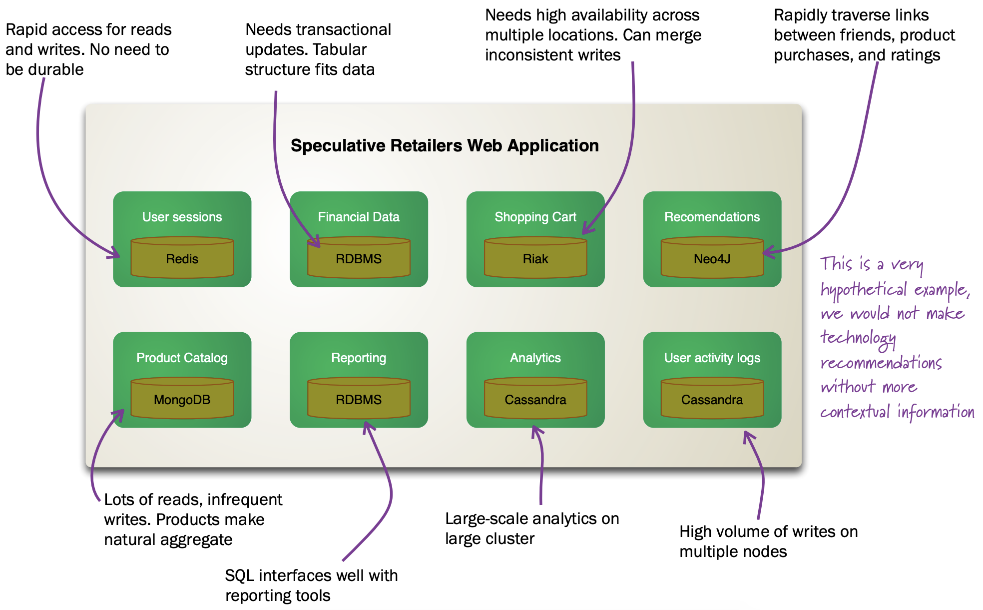
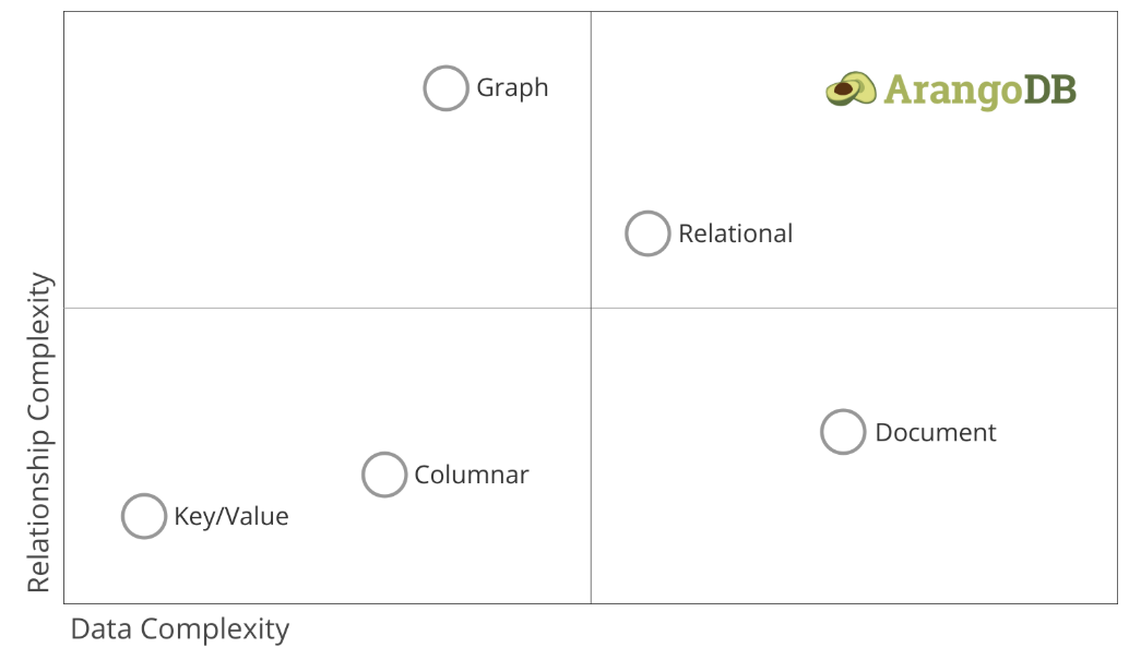
So does this mean that we should leave SQL behind? No. What we’ll be looking at is polyglot persistence: depending on what data you’re working with, some of that might still be stored in an SQL database, while other parts are stored in a document store and graph database (see below). So instead of having a single database, we can end up with a collection of databases to support a single application.
 Source: https://martinfowler.com/articles/nosql-intro-original.pdf
This figure shows how in the hypothetical case of a retailer’s web application we might be using a combination of 8 different database technologies to store different types of information. Note that RDBMS are still part of the picture!
You’ll often hear the term NoSQL as in “No-SQL”, but this should be interpreted as “Not-Only-SQL”.
2. Intermezzo: JSON
Before we proceed, we’ll have a quick look at the JSON (“JavaScript Object Notation”) text format, which is often used in different database systems. JSON follows the same principle as XML, in that it describes the data in the object itself. An example JSON object:
{ code:"I0D54A",
  name:"Big Data",
  lecturer:"Jan Aerts",
  keywords:["data management","NoSQL","big data"],
  students:[
    {student_id:"u0123456", name:"student 1"},
    {student_id:"u0234567", name:"student 2"},
    {student_id:"u0345678", name:"student 3"}]}
JSON has very simple syntax rules:
- Data is in key/value pairs. Each is in quotes, separated by a colon. In some cases you might omit the quotes around the key, but not always.
- Data is separated by commas.
- Curly braces hold objects.
- Square brackets hold arrays.
JSON values can be numbers, strings, booleans, arrays (i.e. lists), objects or NULL; JSON arrays can contain multiple values (including JSON objects); JSON objects contain one or more key/value pairs.
These are two JSON arrays:
["data management","NoSQL","big data"]

[{student_id:"u0123456", name:"student 1"},
 {student_id:"u0234567", name:"student 2"},
 {student_id:"u0345678", name:"student 3"}]
And a simple JSON object:
{student_id:"u0345678", name:"student 3"}And objects can be nested as in the first example.
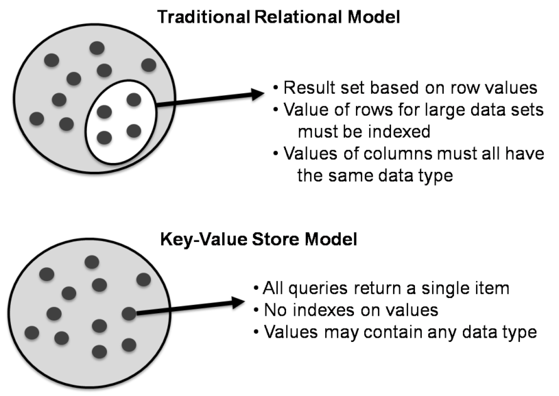
3. Key-value stores
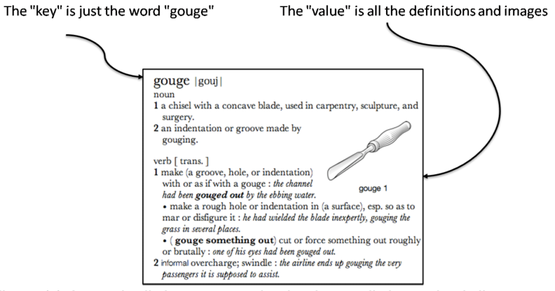
Key/value stores are a very simple type of database. The only thing they do, is link an arbitrary blob of data (the value) to a key (a string). This blob of data can be a piece of text, an image, etc. It is not possible top run queries. Key-value stores therefore basically act as dictionaries:
A key/value store only allows 3 operations: put, get and delete. Again: you can not query.
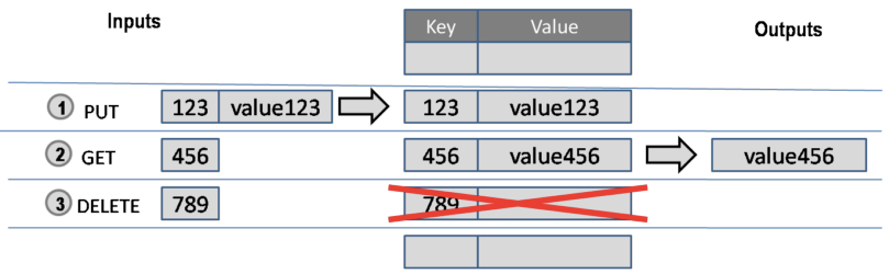
For example:
This type of database is very scalable, and allows for fast retrieval of values regardless of the number of items in the database. In addition, you can store whatever you want as a value; you don’t have to specify the data type for that value.
There basically exist only 2 rules when using a key/value store:
- Keys should be unique: you can never have two things with the same key.
- Queries on values are not possible: you cannot select a key/value pair based on something that is in the value. This is different from e.g. a relational database, where you use a
WHEREclause to constrain a result set. The value should be considered as opaque.
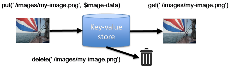
Although (actually: because) they are so simple, there are very specific use cases for key/value stores, for example to store webpages: the key is the URL, the value is the HTML. If you go to a webpage that you visited before, your web browser will first check if it has stored the contents of that website locally beforehand, before doing the costly action of downloading the webpage over the internet.
3.1 Implementations
Many implementations of key/value stores exist, probably the easiest to use being Redis (http://redis.io). Try it out on http://try.redis.io. ArangoDB is a multi-model database which also allows to store key/values (see below).
4. Document-oriented databases
In contrast to relational databases (RDBMS) which define their columns at the table level, document-oriented databases (also called document stores) define their fields at the document level. You can imagine that a single row in a RDBMS table corresponds to a single document where the keys in the document correspond to the column names in the RDBMS. Let’s look at an example table in a RDBMS containing information about buildings:
| id | name | address | city | type | nr_rooms | primary_or_secondary |
|---|---|---|---|---|---|---|
| 1 | building1 | street1 | city1 | hotel | 15 | |
| 2 | building2 | street2 | city2 | school | primary | |
| 3 | building3 | street3 | city3 | hotel | 52 | |
| 4 | building4 | street4 | city4 | church | ||
| 5 | building5 | street5 | city5 | house | ||
| … | … | … | … | … | … | … |
This is a far from ideal way for storing this data because many cells will remain empty based on the type of building their rows represent: the primary_or_secondary column will be empty for every single building except for schools. Also: what if we want to add a new row for a type of building that we don’t have yet? For example: a shop for which we also need to store the weekly closing day. To be able to do that, we’d need to first alter the whole table by adding a new column.
In document-oriented databases, these keys are however stored with the documents themselves. A typical way to represent this is as in JSON format, and can be represented as such:
[
  { id: 1,
    name: "building1",
    address: "street1",
    city: "city1",
    type: "hotel",
    nr_rooms: 15 },
  { id: 2,
    name: "building2",
    address: "street2",
    city: "city2",
    type: "school"
    primary_or_secondary: "primary" },
  { id: 3,
    name: "building3",
    address: "street3",
    city: "city3",
    type: "hotel",
    nr_rooms: 52 },
  { id: 4,
    name: "building4",
    address: "street4",
    city: "city4",
    type: "church" },
  { id: 5,
    name: "building5",
    address: "street5",
    city: "city5",
    type: "house" },
  { id: 6,
    name: "building6",
    address: "street6",
    city: "city6",
    type: "shop",
    closing_day: "Monday" }
]
Notice that in the document for a house (id of 5), there is no mention of primary_of_secondary because it is not relevant as it is for a hotel.
4.1 Nomenclature
The way that things are named in document stores is a bit different than in RDBMS, but in general a collection in a document store corresponds to a table in a RDBMS, and a document corresponds to a row.
4.2 Joining vs embedding
Whereas you use a table join in a RDBMS to combine different concepts/tables, you’d use linking (which is equivalent to a join) or embedding in document stores.
A table join in RDBMS:
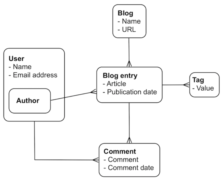
Linking and embedding in a document store:
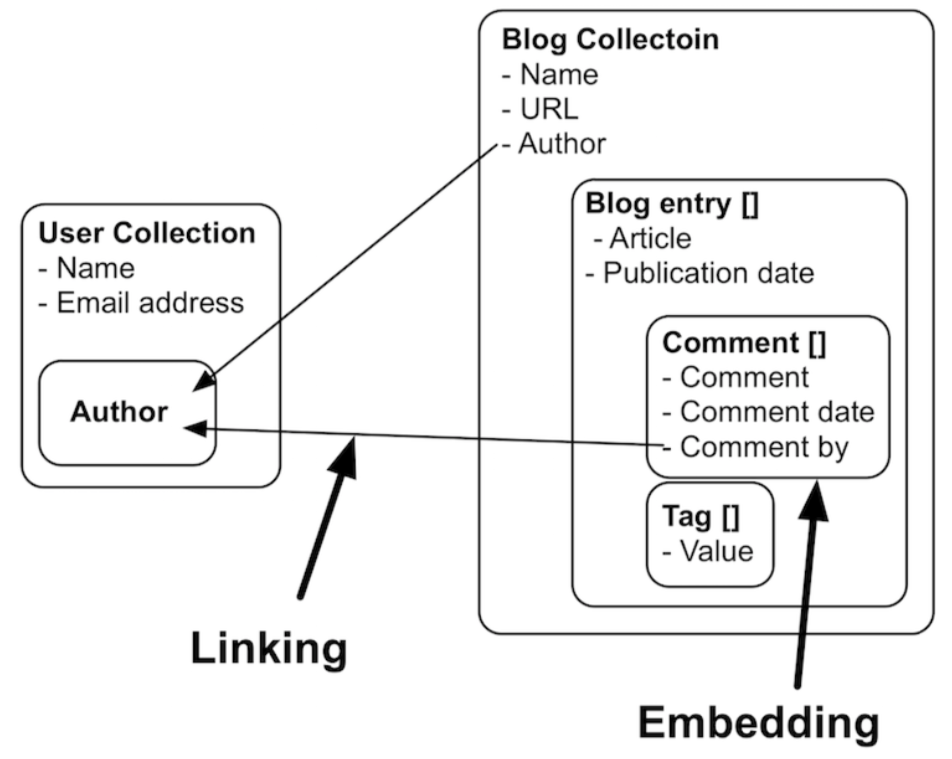
This fact that we can use embedding has multiple advantages:
- The embedded objects are returned in the same query as the parent object, meaning that only 1 trip to the database is necessary. In the example above, if you’d query for a blog entry, you get the comments and tags with it for free.
- Objects in the same collection are generally stored sequentially on disk, leading to fast retrieval.
- If the document model matches your domain, it is much easier to understand than a normalised relational database.
In specific document-oriented databases like MongoDB, the fact that you start linking between documents should give you some code smell. This is because in MongoDB you cannot query documents and follow links between collections. This will have to be done in your (R, python, or other) application code. (This is actually one of the advantages of a multi-model database like ArangoDB which does make this possible.)
4.3 Difference with key/value stores
In a way, document stores are similar to key/value stores. You could think of the automatically generated key in the document store to resemble the key in the key/value store, and the rest of the document being the value. However, there is a major difference: in key/value stores, documents can only be retrieved using their key and the documents are not searchable themselves. In contrast, the key in document stores is almost never used explicitely of even seen.
4.4 Data modelling
The data model depends on your use case, and your choice will greatly affect the complexity and performance of the queries. Let’s for example look at the genotypes from the previous session. There are 2 options to choose between: you can create documents per individual, or per SNP.
Per individual, a document could look like this:
{ name: "Tom",
  ethnicity: "African",
  genotypes: [
    { snp: "rs0001",
      genotype: "A/A",
      position: "1_8271" },
    { snp: "rs0002",
      genotype: "A/G",
      position: "1_127279" },
    { snp: "rs0003",
      genotype: "C/C",
      position: "1_82719" },
    ...
  ]}
{ name: "John",
  ethnicity: "Caucasian",
  ...
In contrast, a document per SNP looks like:
{ snp: "rs0001",
  position: "1_8271",
  genotypes: [
    { name: "Tom",
      ethnicity: "African",
      genotype: "A/A" },
    { name: "John",
      ethnicity: "Caucasian",
      genotype: "A/A" },
    ...
  ]}
We’ll go into loading data into and querying data from a document-related database later.
If your data documents are structured along individuals, it will bve cvery fast to get all genotypes for a given individual, but very slow to get all genotypes for a given SNP. Therefore, in a big data setting, it is not unusual to have both, and to generate one of these collections based on the other.
4.5 Implementations
Probably the best known document store is mongodb (http://mongodb.com). This database system is single-model in that it does not handle key/values and graphs; it’s only meant for storing documents.
5. Graph databases
Graphs are used in a wide range of applications, from fraud detection (see the Panama Papers) and anti-terrorism and social marketing to drug interaction research and genome sequencing.
Graphs or networks are data structures where the most important information is the relationship between entities rather than the entities themselves, such as friendship relationships. Whereas in relational databases you typically aggregate operations on sets, in graph databases you’ll more typically hop around relationships between records. Graphs are very expressive, and any type of data can be modelled as one (although that is no guarantee that a particular graph is fit for purpose).
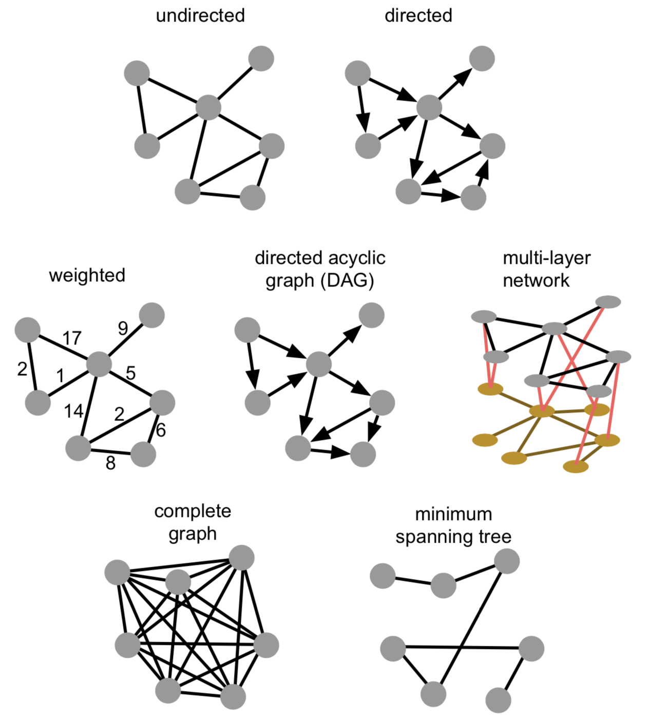
Graphs come in all shapes and forms. Links can be directed or undirected, weighted or unweighted. They can be directed acyclic graphs (where no loops exist), consist of one or more connected components, and actually consist of multiple graphs themselves. The latter (so-called multi-layer networks) can e.g. be a first network representing friendships between people, a second network representing cities and how they are connected through public transportation, and both being linked by which people work in which cities.
5.1 Nomenclature
A graph consists of vertices (aka nodes, aka objects) and edges (aka links, aka relations), where an edge is a connection between two vertices. Both vertices and edges can have properties.
\[G = (V,E)\]Any graph can be described using different metrics:
- order of a graph = number of nodes
- size of a graph = number of edges
- graph density = how much its nodes are connected. In a dense graph, the number of edges is close to the maximal number of edges (i.e. a fully-connected graph).
- for undirected graphs, this is: \(\frac{2 |E|}{|V|(|V|-1)}\)
- for directed graphs, this is: \(\frac{|E|}{|V|(|V|-1)}\)
- the degree of a node = how many edges are connected to the node. This can be separated into in-degree and out-degree, which are - respectively - the number of incoming and outgoing edges.
- the distance between two nodes = the number of edges in the shortest path between them
- the diameter of a graph = the maximum distance in a graph
- a d-regular graph = a graph where the maximum degree is the same as the minimum degree d
- a path = a sequence of edges that connects a sequence of different vertices
- a connected graph = a graph in which there exists a direct connection between any two vertices
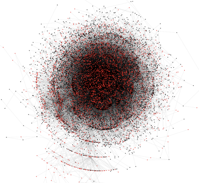
5.2 Centralities
Another important way of describing nodes is based on their centrality, i.e. how central they are in the network. There exist different versions of this centrality:
- degree centrality: how many other vertices a given vertex is connected to. This is the same as node degree.
- betweenness centrality: how many critical paths go through this node? In other words: without these nodes, there would be no way for to neighbours to communicate.
, where the denominator is the number of vertex pairs excluding the vertex itself. \(g_jk(i)\) is number of shortest paths between \(j\) and \(k\), going through i; \(g_jk\) is the total number of shortest paths between \(j\) and \(k\).
- closeness centrality: how much is the node in the “middle” of things, not too far from the center. This is the inverse total distance to all other nodes.
In the image below, nodes in A are coloured based on betweenness centrality, in B based on closeness centrality, and in D on degree centrality.
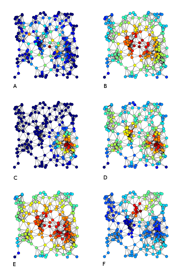
Source of image: to add
5.3 Graph mining
Graphs are very generic data structures, but are amenable to very complex analyses. These include the following.
Community detection
A community in a graph is a group of nodes that are densely connected internally. You can imagine that e.g. in social networks we can identify groups of friends this way.
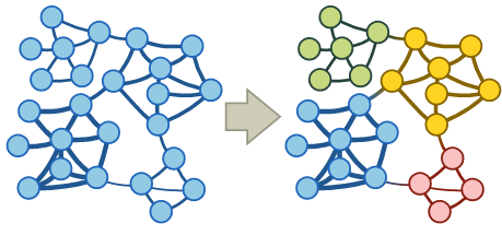
Several approaches exist to finding communities:
- null models: a community is a set of nodes for which the connectivity deviates the most from the null model
- block models: identify blocks of nodes with common properties
- flow models: a community is a set of nodes among which a fl�ow persists for a long time once entered
The infomap algorithm is an example of a flow model (for a demo, see http://www.mapequation.org/apps/MapDemo.html).
Link prediction
When data is acquired from a real-world source, this data might be incomplete and links that should actually be there are not in the dataset. For example, you gather historical data on births, marriages and deaths from church and city records. There is therefore a high chance that you don’t have all data. Another domain where this is important is in protein-protein interactions.
Link prediction can be done in different ways, and can happen in a dynamic or static setting. In the dynamic setting, we try to predict the likelihood of a future association between two nodes; in the static setting, we try to infer missing links. These algorithms are based on a similarity matrix between the network nodes, which can take different forms:
- graph distance: the length of the shortest path between 2 nodes
- common neighbours: two strangers who have a common friend may be introduced by that friend
- Jaccard’s coefficient: the probability that 2 nodes have the same neighbours
- frequency-weighted common neighbours (Adamic/Adar predictor): counts common features (e.g. links), but weighs rare features more heavily
- preferential attachment: new link between nodes with high number of links is more likely than between nodes with low number of links
- exponential damped path counts (Katz measure): the more paths there are between two nodes and the shorter these paths are, the more similar the nodes are
- hitting time: random walk starts at node A => expected number of steps required to reach node B
- rooted pagerank: idem, but periodical reset to prevent that 2 nodes that are actually close are connected through long deviation
Subgraph mapping
Subgraph mining is another type of query that is very important in e.g. bioinformatics. Some example patterns:
- [A] three-node feedback loop
- [B] tree chain
- [C] four-node feedback loop
- [D] feedforward loop
- [E] bi-parallel pattern
- [F] bi-fan
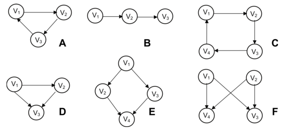
It is for example important when developing a drug for a certain disease by knocking out the effect of a gene that that gene is not in a bi-parallel pattern (V2 in image E above) because activation of node V4 is saved by V3.
5.4 Data modelling
In general, vertices are used to represent things and edges are used to represent connections. Vertex properties can include e.g. metadata such as timestamp, version number etc; edges properties often include the weight of a connection, but can also cover things like the quality of a relationship and other metadata of that relationship.
Below is an example of a graph:
Basically all types of data can be modelled as a graph. Consider our buildings table from above:
| id | name | address | city | type | nr_rooms | primary_or_secondary |
|---|---|---|---|---|---|---|
| 1 | building1 | street1 | city1 | hotel | 15 | |
| 2 | building2 | street2 | city2 | school | primary | |
| 3 | building3 | street3 | city3 | hotel | 52 | |
| 4 | building4 | street4 | city4 | church | ||
| 5 | building5 | street5 | city5 | house | ||
| … | … | … | … | … | … | … |
This can also be represented as a network, where:
- every building is a vertex
- every value for a property is a vertex as well
- the column becomes the relation
For example, the information for the first building can be represented as such:

There is actually a formal way of describing this called RDF, but we won’t go into that here…
6. ArangoDB - a multi-model database
As for RDBMS, there are many different implementations of document-oriented databases. Unfortunately, as the NoSQL field is much younger than the RDBMS area, things have not settled enough so that standards are formed. In the RDBMS world, there are many implementations such as Oracle, MySQL, PostgreSQL, Microsoft Access, etc, but they all conform to the same standard for querying their data: SQL. In the NoSQL world, however, this is very different and different implementations use very different query languages. For example, a search in the document store MongoDB (which is widely used) looks like this:
db.individuals.findAll({ethnicity: "African"}, {genotypes: 1})whereas it would look like this in ArangoDB:
FOR i IN individuals
FILTER i.ethnicity = 'African'
RETURN i.genotypes
The same is true for graph databases. A query in the popular Neo4j database can look like this (in what is called the cypher language):
MATCH (a)-[:WORKS_FOR]->(b:Company {name: "Microsoft"}) RETURN awould be the following in gremlin:
g.V().out('works_for').inV().hasLabel("Company").has("name", "Microsoft")whereas it would look like this in ArangoDB (in AQL):
FOR a IN individuals
  FOR v,e,p IN 1..1 OUTBOUND a GRAPH 'works_for'
    FILTER v.name = 'Microsoft'
    RETURN a
Further in this post we’ll be using ArangoDB as our database, because - for this course - we can then at least stick with one query language.
6.1 Starting with ArangoDB
We will first need to install ArangoDB. It is available on a variety of operating systems and can be downloaded from https://www.arangodb.com/download-major/.
For getting started with ArangoDB, see here. Some of the following is extracted from that documentation. After installing ArangoDB, you can access the web interface at http://localhost:8529; log in as user root (without a password) and connect to the _system database. (Note that in a real setup, the root user would only be used for administrative purposes, and you would first create a new username. For the sake of simplicity, we’ll take a shortcut here.)
Web interface vs arangosh
In the context of this course, we will use the web interface for ArangoDB. Although very easy to use, it does have some shortcomings compared to the command line arangosh, or using ArangoDB from within programs written in python or other languages. For example, we won’t be able to run centrality queries using the web interface. If you’re even a little bit serious about using databases, you should get yourself acquainted with the shell as well.
6.2 Loading data
Document data
Let’s load some data. Download the list of airports in the US from http://vda-lab.be/assets/airports.json. This file looks like this:
{"_key": "00M", "name": "Thigpen ", "city": "Bay Springs", "state": "MS", "country": "USA", "lat": 31.95376472, "long": "Thigpen ", "vip": false}
{"_key": "00R", "name": "Livingston Municipal", "city": "Livingston", "state": "TX", "country": "USA", "lat": 30.68586111, "long": "Livingston Municipal", "vip": false}
{"_key": "00V", "name": "Meadow Lake", "city": "Colorado Springs", "state": "CO", "country": "USA", "lat": 38.94574889, "long": "Meadow Lake", "vip": false}
...
Remember from above that document databases often use JSON as their format. To load this into ArangoDB:
- Create a new collection (
Collections->Add Collection) with the nameairports. Thetypeshould bedocument.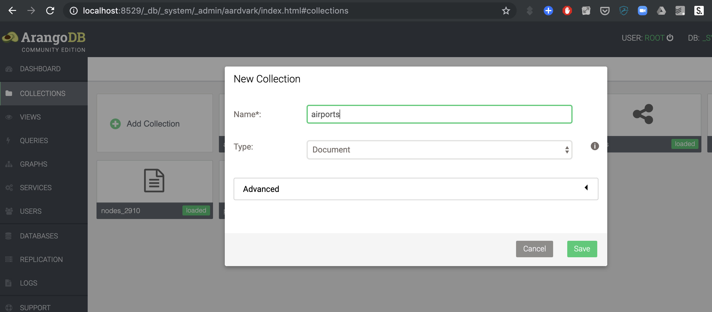
- Click on the collection, and then the
Upload documents from JSON filebutton at the top.
- Select the
airports.jsonfile that you just downloaded onto your computer.
You should end up with something like this:
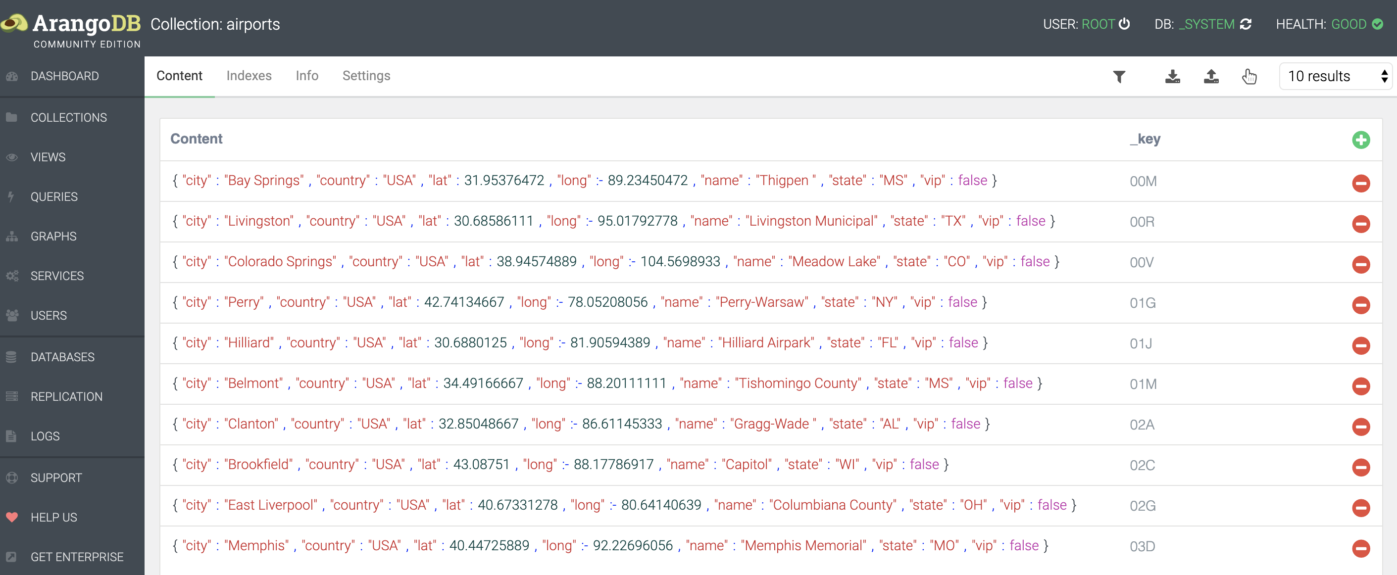
Notice that every document has a _key defined.
Link data
In addition to _key, ArangoDB documents can have other special keys. In a graph context, links are nothing more than regular documents, but which have a _from and _to key to refer to other documents that are the nodes. So links in ArangoDB are basically also just documents, but with the special keys _from and _to. This means that we can also query them as documents (which is what we will actually do in “6.2 Querying document data”).
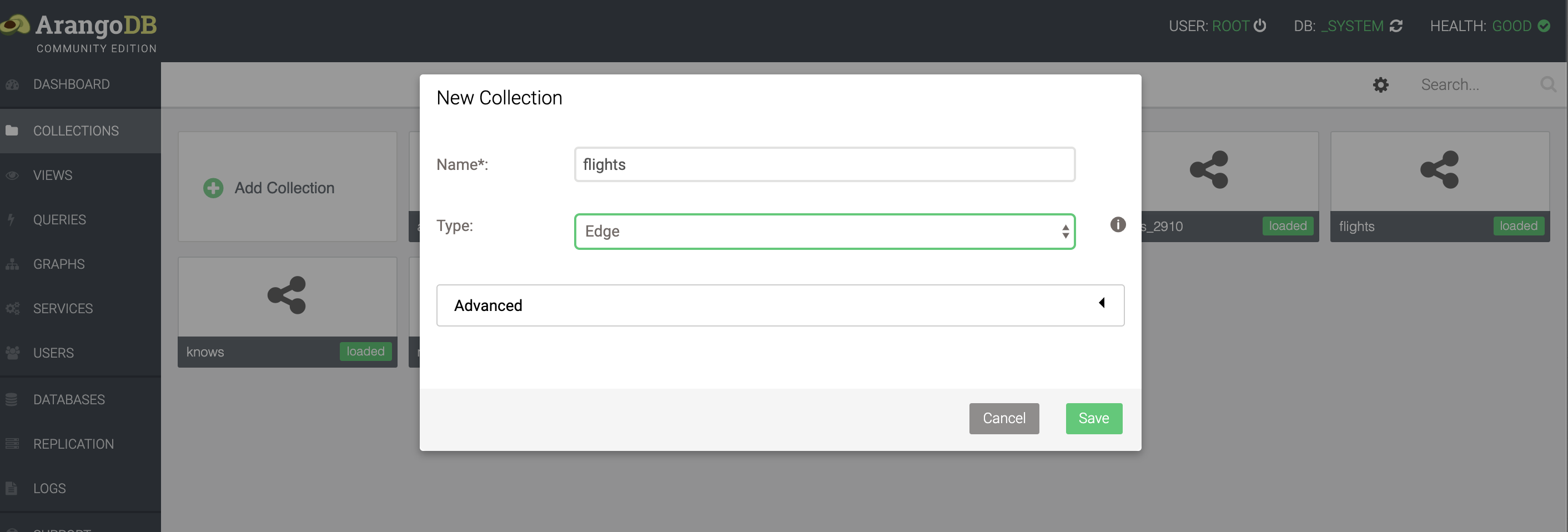
We have a flight dataset, that you can download from here. Similar to loading the airports dataset, we go to the Collections page in the webinterface, and click Upload. This time, however, we need to set the type to Edge rather than Document.
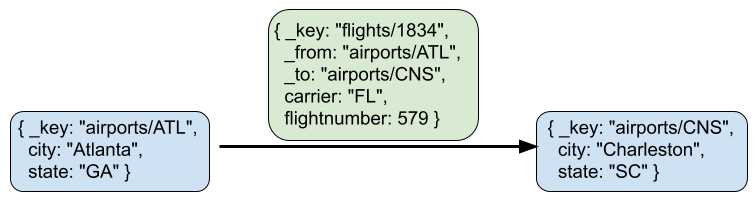
This is what a single flight looks like:
{
  "_key": "1834",
  "_id": "flights/1834",
  "_from": "airports/ATL",
  "_to": "airports/CHS",
  "_rev": "_ZRp7f-S---",
  "Year": 2008,
  "Month": 1,
  "Day": 1,
  "DayOfWeek": 2,
  "DepTime": 2,
  "ArrTime": 57,
  "DepTimeUTC": "2008-01-01T05:02:00.000Z",
  "ArrTimeUTC": "2008-01-01T05:57:00.000Z",
  "UniqueCarrier": "FL",
  "FlightNum": 579,
  "TailNum": "N937AT",
  "Distance": 259
}
6.3 Querying key/values: ArangoDB as a key/value store
As mentioned above, key/value stores are very quick for returning documents given a certain key. ArangoDB can be used as a key/value store as well. Remember from above that a key/value store should only do these things:
- Create a document with a given key
- Return a document given a key
- Delete a document given a key
Let’s try these out. But before we do so, it’d be cleaner if we created a new collection just for this purpose. Go to Collections and create a new collection named keyvalues.
ArangoDB uses its own query language, called AQL, to access the data in the different collections. Go to the Queries section in the web interface.
Creating a key/value pair
INSERT {_key: "a", value: "some text"} INTO keyvaluesThis created our first key/value pair! The value can be anything, as we mentioned above:
INSERT {_key: "b", value: [1,2,3,4,5]} INTO keyvalues
INSERT {_key: "c", value: {first: 1, second: 2}} INTO keyvalues
Retrieving a key/value pair
To retrieve a document given a certain key (in this case “c”), we can run the query
RETURN DOCUMENT('keyvalues/c').valueHow this works will get much more clear as we move further down in this post…
Removing a key/value pair
To remove a key/value pair (e.g. the pair for key b), we run the following:
REMOVE b FROM keyvaluesRetrieving and removing key/value pairs are very fast in ArangoDB, because the _key attribute is indexed by default.
6.4 Querying document data: ArangoDB as a document store
Having stored our data in the airports and flights collections, we can query these in the Query section. An overview of the possible high-level operations can be found here: https://www.arangodb.com/docs/stable/aql/operations.html. From that website:
FOR: Iterate over a collection or View, all elements of an array or traverse a graphRETURN: Produce the result of a query.FILTER: Restrict the results to elements that match arbitrary logical conditions.SEARCH: Query the (full-text) index of an ArangoSearch ViewSORT: Force a sort of the array of already produced intermediate results.LIMIT: Reduce the number of elements in the result to at most the specified number, optionally skip elements (pagination).LET: Assign an arbitrary value to a variable.COLLECT: Group an array by one or multiple group criteria. Can also count and aggregate.
We’ll go over some of these below.
Note: When in the following section I write something like “equivalent in SQL” with an actual SQL query, this will actually be hypothetical. In other words: you cannot run that actual query on the ArangoDB database as that would not work. It would work if you’d first make an SQL database (e.g. using sqlite as seen in the previous session) and created the necessary tables and rows…
RETURNing a result
The most straightforward way to get a document is to select it by key. When doing this, you have to prepend the key with the name of the collection:
RETURN DOCUMENT("airports/JFK")The above basically treats the ArangoDB database as a key/value store.
You can also get multiple documents if you provide an array of keys instead of a single one:
RETURN DOCUMENT(["airports/JFK","airports/03D"])Notice the square brackets around the keys!
FOR: Looping over all documents
Remember that in SQL, a query looked like this:
SELECT state
FROM airports
WHERE lat > 35;
SQL is a declarative language, which means that you tell the RDBMS what you want, not how to get it. This is not exactly true for AQL, which does need you to specify that you want to loop over all documents. The same query as the SQL one above in AQL would be:
FOR a IN airports
  FILTER a.lat > 35
  RETURN a
Similarly, the minimal SQL query is:
SELECT * FROM airports;, whereas the minimal AQL query is:
FOR a IN airports
  RETURN a
You can nest FOR statements, in which case you’ll get the cross project:
FOR a IN [1,2,3]
  FOR b IN [10,20,30]
    RETURN [a, b]
This will return:
1  10
2  10
3  10
1  20
2  20
3  20
1  30
2  30
3  30
If you don’t want to return the whole document, you can specify this in the RETURN statement. This is called a projection. For example:
FOR a IN airports
  RETURN a.name
or
FOR a IN airports
  RETURN { "name": a.name, "state": a.state }
This is equivalent to specifying the column names in an SQL query:
SELECT name, state
FROM airports;
Returning only DISTINCT results
FOR a IN airports
RETURN DISTINCT a.stateFILTERing documents
Data can be filtered using FILTER:
FOR a IN airports
  FILTER a.state == 'CA'
  RETURN a
To combine different filters, you can use AND and OR:
FOR a IN airports
  FILTER a.state == 'CA'
  AND a.vip == true
  RETURN a
FOR a IN airports
FILTER a.state == 'CA'
OR a.vip == true
RETURN aIt is often recommended to use parentheses to clarify the order of the filters:
FOR a IN airports
  FILTER ( a.state == 'CA' OR a.vip == true )
  RETURN a
Instead of AND, you can also apply multiple filters consecutively:
FOR a IN airports
  FILTER a.state == 'CA'
  FILTER a.vip == true
RETURN aSORTing the results
FOR a IN airports
  SORT a.lat
  RETURN [ a.name, a.lat ]
As in SQL, AQL allows you do sort in descending order:
FOR a IN airports
  SORT a.lat DESC
  RETURN [ a.name, a.lat ]
Combining different filters, limits, etc
Remember that in SQL, you can combine different filters, sortings etc.
In SQL:
SELECT * FROM airports
WHERE a.state = 'CA'
AND a.lat > 20
AND vip = true
SORT BY lat
LIMIT 15;
In AQL, the different filters, sorts, limits, etc are applied top to bottom. This means that the following two do not necessarily give the same results:
FOR a IN airports
  FILTER a.vip == true
  FILTER a.state == 'CA'
  LIMIT 5
  RETURN a
FOR a IN airports
FILTER a.vip == true
LIMIT 5
FILTER a.state == 'CA'
RETURN aFunctions in ArangoDB
ArangoDB includes a large collections of functions that can be run at different levels, e.g. to analyse the underlying database, to calculate aggregates like minimum and maximum from an array, to calculating the geographical distance between two locations on a map, to concatenate strings, etc. For a full list of functions see https://www.arangodb.com/docs/stable/aql/functions.html.
Let’s have a look at some of these.
CONCAT and CONCAT_SEPARATOR
Using CONCAT and CONCAT_SEPARATOR we can return whole strings instead of just arrays and documents.
FOR f IN flights
  LIMIT 10
  RETURN [f.FlightNum, f._from, f._to]
FOR f IN flights
LIMIT 10
RETURN CONCAT("Flight ", f.FlightNum, " departs from ", f._from, " and goes to ", f._to, ".")returns
[
"Flight 579 departs from airports/ATL and goes to airports/CHS.",
"Flight 2895 departs from airports/CLE and goes to airports/SAT.",
"Flight 7185 departs from airports/IAD and goes to airports/CLE.",
"Flight 859 departs from airports/JFK and goes to airports/PBI.",
"Flight 5169 departs from airports/CVG and goes to airports/MHT.",
"Flight 9 departs from airports/JFK and goes to airports/SFO.",
"Flight 1831 departs from airports/MIA and goes to airports/TPA.",
"Flight 5448 departs from airports/CVG and goes to airports/GSO.",
"Flight 878 departs from airports/FLL and goes to airports/JFK.",
"Flight 680 departs from airports/TPA and goes to airports/PBI."
]
Something similar can be done with providing a separator. This can be useful when you’re creating a comma-separated file.
FOR f IN flights
  LIMIT 10
  RETURN CONCAT_SEPARATOR(' -> ', f._from, f._to)
returns
[
"airports/ATL -> airports/CHS",
"airports/CLE -> airports/SAT",
"airports/IAD -> airports/CLE",
"airports/JFK -> airports/PBI",
"airports/CVG -> airports/MHT",
"airports/JFK -> airports/SFO",
"airports/MIA -> airports/TPA",
"airports/CVG -> airports/GSO",
"airports/FLL -> airports/JFK",
"airports/TPA -> airports/PBI"
]
MIN and MAX
These functions do what you expect them to do. See later in this post when we’re looking at aggregation.
RETURN MAX([1,5,20,1,4])Subqueries
Remember that in SQL, we can replace the table mentioned in the FROM clause with a whole SQL statement, something like this:
SELECT COUNT(*) FROM (
  SELECT name FROM airports
  WHERE state = 'TX');
We can do something similar with AQL. For argument’s sake, let’s wrap a simple query into another one which just returns the result of the inner query:
FOR s IN (
    FOR a IN airports
        COLLECT state = a.state WITH COUNT INTO nrAirports
        SORT nrAirports DESC
        RETURN {
            "state" : state,
            "nrAirports" : nrAirports
        }
    )
RETURN s
This is exactly the same as if we would have run only the inner query. An AQL query similar to the SQL query above:
FOR airport IN (
    FOR a IN airports
        FILTER a.state == "TX"
        RETURN a
    )
    COLLECT WITH COUNT INTO c
    RETURN c
Joining collections
It is simple enough to combine different collections, just by nesting FOR loops but making sure that there exits a FILTER in the inner loop to match up IDs. For example, to list all destination airports and distances for flights where the departure airport lies in California:
FOR a IN airports
  FILTER a.state == 'CA'
  FOR f IN flights
    FILTER f._from == a._id
    RETURN DISTINCT {departure: a._id, arrival: f._to, distance: f.Distance}
Gives:
airports/ACV  airports/SFO  250
airports/ACV  airports/SMF  207
airports/ACV  airports/CEC  56
...
(Remember from above that using links in a document setting consitute a code smell. If you’re doing this a lot, check if your data should be modelled as a graph. Further down when we’re talking about ArangoDB as a graph database we’ll write a version of this same query that uses a graph approach.)
What if we want to show the departure and arrival airports full names instead of their codes, and have an additional filter on the arrival airport? To do this, we need an additional join with the airports table:
FOR a1 IN airports
  FILTER a1.state == 'CA'
  FOR f IN flights
    FILTER f._from == a1._id
    FOR a2 in airports
      FILTER a2._id == f._to
      FILTER a2.state == 'CA'
      RETURN DISTINCT {
        departure: a1.name,
        arrival: a2.name,
        distance: f.Distance }
This will return something like the following:
Arcata  San Francisco International  250
Arcata  Sacramento International     207
Arcata  Jack McNamara                 56
...
The above joins are inner joins, which means that we will only find the departure airports for which such arrival airports exist (see the SQL session). What if we want to list the airports in California that do not have any flights to other airports in California? In this case, put the second FOR loop within the RETURN statement:
FOR a1 IN airports
  FILTER a1.state == 'CA'
  RETURN {
    departure: a1.name,
    arrival: (
        FOR f IN flights
            FILTER f._from == a1._id
            FOR a2 in airports
                FILTER a2._id == f._to
                FILTER a2.state == 'CA'
                RETURN DISTINCT a2.name
                )}
This returns:
...
Buchanan         []
Jack McNamara    ["San Francisco International","Arcata"]
Chico Municipal  ["San Francisco International"]
Camarillo        []
...
You’ll see that e.g. Buchanan and Camarillo are also listed, which was not the case before.
Grouping
To group results, AQL provides the COLLECT keyword. Note that this does grouping, but no aggregation. With COLLECT you create a new variable that will be used for the grouping.
FOR a IN airports
  COLLECT state = a.state INTO airportsByState
  RETURN {
    "state" : state,
    "airports" : airportsByState
  }
This code goes through each airport, and collects the state that it’s in. It’ll return a list of states with for each the list of their airports:
[
  {
    "state": "AK",
    "airports": [
      {
        "a": {
          "_key": "0AK",
          "_id": "airports/0AK",
          "_rev": "_ZYukZZy--e",
          "name": "Pilot Station",
          "city": "Pilot Station",
          "state": "AK",
          "country": "USA",
          "lat": 61.93396417,
          "long": "Pilot Station",
          "vip": false
        }
      },
      {
        "a": {
          "_key": "15Z",
          "_id": "airports/15Z",
          "_rev": "_ZYukZa---I",
          "name": "McCarthy 2",
          "city": "McCarthy",
          "state": "AK",
          "country": "USA",
          "lat": 61.43706083,
          "long": "McCarthy 2",
          "vip": false
        }
      },
      ...
The a in the output above refers to the FOR a IN airports. Using FOR x IN airports would have used x for each of the subdocuments above.
This output is however not ideal… We basically just want to have the airport codes instead of the complete document.
FOR a IN airports
  COLLECT state = a.state INTO airportsByState
  RETURN {
    "state" : state,
    "airports" : airportsByState[*].a._id
  }
This results in:
state  airports
AK     ["airports/0AK","airports/15Z","airports/16A","airports/17Z", ...]
AL     ["airports/02A","airports/06A","airports/08A","airports/09A", ...]
...
What is this [*].a._id? If we look at the output from the previous query, we get the full document for each airport, and the form of the output is:
[
  {
    "state": "AK",
    "airports": [
      {
        "a": {..., "_id": "airports/0AK", ...}
      },
      {
        "a": {...,"_id": "airports/15Z", ...}
      },
      ...]
  }
]
The [*].a._id means “for each of these (*), return the value for a._id”. This is very helpful if you want to extract a certain key from an array of documents.
COLLECT can be combined with the WITH COUNT pragma to return the number of items, for example:
FOR a IN airports
  COLLECT state = a.state WITH COUNT INTO nrAirports
  SORT nrAirports DESC
  RETURN {
    "state" : state,
    "nrAirports" : nrAirports
  }
AK 263
TX 209
CA 205
...The above corresponds to the following in SQL:
SELECT state, count(*)
FROM airports
GROUP BY state;
Another example: how many flights does each carrier have?
FOR f IN flights
    COLLECT carrier = f.UniqueCarrier WITH COUNT INTO c
    SORT c DESC
    LIMIT 3
    RETURN {
        carrier: carrier,
        nrFlights: c
    }
The answer:
carrier  nrFlights
WN       48065
AA       24797
OO       22509
Apparently SouthWest Airlines (WN) has many more domestic flights than any other airline, including American Airlines (AA) and … (I don’t know what the OO stands for…)
Aggregation
We can go further and make calculations as well. Note that we can only use AGGREGATE when we have run COLLECT before. When using AGGREGATE we create a new variable and assign it a value using one of the functions that we saw here.
What is the average flight distance?
FOR f IN flights
    COLLECT AGGREGATE
    avg_length = AVG(f.Distance)
    RETURN avg_length
The answer is 729.93 kilometers.
What is the shortest flight for each day of the week?
FOR f IN flights
  COLLECT dayOfWeek = f.DayOfWeek
  AGGREGATE minDistance = MIN(f.Distance)
  RETURN {
    "dow" : dayOfWeek,
    "minDistance": minDistance
  }
Based on this query, we see that there is actually a flight on Wednesday that is shorter than any other flight.
dow minDistance
1 31
2 30
3 24
4 31
5 31
6 31
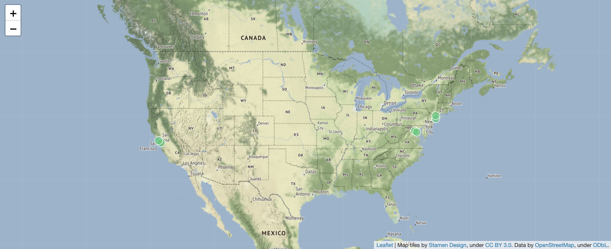
7 30OK, now we’re obviously interested in what those shortest flights are. Given what we have seen above, this will give us a map with those flights. For a geographical query, ArangoDB uses OpenStreetMap to visualise the returned points:
FOR f IN flights
  SORT f.Distance
  LIMIT 3
  LET myAirports = [DOCUMENT(f._from), DOCUMENT(f._to)]
  FOR a IN myAirports
    RETURN GEO_POINT(a.long, a.lat)
Here we used the LET operation (see above “Querying document data”) for creating an array with two documents that we can loop over in the next lines using FOR.
Intermezzo: now we’re curious: what actually are the names of the airports with the shortest flight? (They should be included in the picture above, right?)
FOR f IN flights
    SORT f.Distance
    LIMIT 1
    LET from = (
        FOR a IN airports
        FILTER a._id == f._from
        RETURN a.name )
    LET to = (
        FOR a IN airports
        FILTER a._id == f._to
        RETURN a.name )
    RETURN [from[0], to[0], f.Distance]
Result:
[
  [
    "Washington Dulles International",
    "Ronald Reagan Washington National",
    24
  ]
]
6.5 Querying link data: ArangoDB as a graph store
Although both airports and flights are collections in ArangoDB, we set flights to be an “Edge” collection, which means that it should have a _from and a _to key as it is used to link documents in other collections to each other.
There are 2 types of graphs in ArangoDB: named graphs and anonymous graphs.
Before we run the queries below, we will first create a named graph. To do so, click on Graphs and then on Add Graph. You will be presented with the following box:
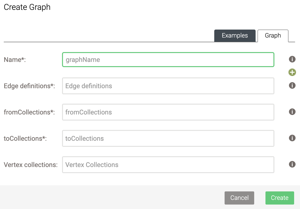
Here, select the following:
- Name: flightsGraph
- Edge definitions: flights
- fromCollections: airports
- toCollections: airports
- Leave Vertex collections empty.
Graph queries
Of course what are we with graphs if we can’t ask graph-specific questions. At the beginning of this post, we looked at how difficult it was to identify all friends of friends of James. What would this look like in a graph database?
The FOR syntax looks a little different when you’re querying a graph rather than a collection of documents. It’s
FOR v,e,p IN 2..2 ANY "myKey" GRAPH "myGraph"
LIMIT 5
RETURN v._id
This means (going from right to left):
- take the graph
myGraph - start from the document with
_keyofmyKey - follow links in both directions (
ANYis bothINBOUNDandOUTBOUND) - for 2 steps (
2..2meansmin..max) - take the final vertex
v, the last link that lead to ite, and the whole pathpfrom start to finish - and return the final vertex’s id
The whole path p contains the full list of vertices from source to target, as well as the list of edges between them.
Note that the key graph need to be in quotes. The result of the query
FOR v,e,p IN 2..2 ANY "airports/JFK" GRAPH "flights"
LIMIT 5
RETURN v._id
is:
[
  "airports/IAH",
  "airports/JFK",
  "airports/CLT",
  "airports/EWR",
  "airports/ATL"
]
This query is lightning fast compared to what we did with the friends of a friend using a relational database!!
Of course you can add additional filters as well, for example to only return those that are located in California:
FOR v,e,p IN 2..2 ANY 'airports/JFK' GRAPH 'flightsGraph'
LIMIT 5000
FILTER v.state == 'CA'
RETURN DISTINCT v._id
The LIMIT 5000 is so that we don’t go through the whole dataset here, as we’re just running this for demonstration purposes. The result of this query:
[
  "airports/SAN",
  "airports/LAX",
  "airports/ONT",
  "airports/BFL",
  "airports/SNA",
  "airports/SMF",
  "airports/FAT",
  "airports/SBP",
  "airports/PSP",
  "airports/SBA",
  "airports/PMD",
  "airports/MRY",
  "airports/ACV",
  "airports/BUR",
  "airports/CIC",
  "airports/CEC",
  "airports/MOD",
  "airports/RDD"
]
You actually don’t need to create the graph beforehand, and can use the edge collections directly:
FOR v,e,p IN 2..2 ANY 'airports/JFK' flights
LIMIT 5000
FILTER v.state == 'CA'
RETURN DISTINCT v._id
Here we don’t use the keyword GRAPH, collection is not in quotes.
Rewriting the document query that used joins
Above we said that we’d rewrite a query that used the document approach to one that uses a graph approach. The original query listed all airports in California, and listed where any flights were going to and what the distance is.
FOR a IN airports
  FILTER a.state == 'CA'
  FOR f IN flights
    FILTER f._from == a._id
    RETURN DISTINCT {departure: a._id, arrival: f._to, distance: f.Distance}
We can approach this from a graph perspective as well. Instead of checking the _from key in the flights documents, we consider the flights as a graph: we take all Californian airports, and follow all outbound links with a distance of 1.
FOR a IN airports
  FILTER a.state == 'CA'
  FOR v,e,p IN 1..1 OUTBOUND a flights
    RETURN DISTINCT { departure: a._id, arrival: v._id, distance: e.Distance}
This gives the same results.
airports/ACV  airports/SFO  250
airports/ACV  airports/SMF  207
airports/ACV  airports/CEC  56
...
Remember that we actually had quite a bit of work if we wanted to show the airport names instead of their codes:
FOR a1 IN airports
  FILTER a1.state == 'CA'
  FOR f IN flights
    FILTER f._from == a1._id
    FOR a2 in airports
      FILTER a2._id == f._to
      FILTER a2.state == 'CA'
      RETURN DISTINCT {
        departure: a1.name,
        arrival: a2.name,
        distance: f.Distance }
In constrast, we only need to make a minor change in the RETURN statement of the graph query:
FOR a IN airports
  FILTER a.state == 'CA'
  FOR v,e,p IN 1..1 OUTBOUND a flights
    RETURN DISTINCT { departure: a.name, arrival: v.name, distance: e.Distance}
Shortest path
The SHORTEST_PATH function (see here) allows you to find the shortest path between two nodes. For example: how to get in the smallest number of steps from the airport of Pellston Regional of Emmet County (PLN) to Adak (ADK)?
FOR path IN OUTBOUND SHORTEST_PATH 'airports/PLN' TO 'airports/ADK' flights
RETURN path
The result looks like this:
_key  _id           _rev         name                                 city       state  country  lat          long          vip
PLN   airports/PLN  _ZbpOKyy--Q  Pellston Regional of Emmet County    Pellston   MI     USA      45.5709275   -84.796715    false
DTW   airports/DTW  _ZbpOKxu-_S  Detroit Metropolitan-Wayne County    Detroit    MI     USA      42.21205889  -83.34883583  false
IAH   airports/IAH  _ZbpOKyK---  George Bush Intercontinental         Houston    TX     USA      29.98047222  -95.33972222  false
ANC   airports/ANC  _ZbpOKxW-Am  Ted Stevens Anchorage International  Anchorage  AK     USA      61.17432028  -149.9961856  false
ADK   airports/ADK  _ZbpOKxW--o  Adak                                 Adak       AK     USA      51.87796389  -176.6460306  false
The above does not take into account the distance that is flown. We can add that as the weight:
FOR path IN OUTBOUND SHORTEST_PATH 'airports/PLN' TO 'airports/ADK' flights
OPTIONS {
  weightAttribute: "Distance"
}
RETURN path
This shows that flying of Minneapolis instead of Houston would cut down on the number of miles flown:
_key  _id           _rev         name                                 city         state  country  lat          long          vip
PLN   airports/PLN  _ZbpOKyy--Q  Pellston Regional of Emmet County    Pellston     MI     USA      45.5709275   -84.796715    false
DTW   airports/DTW  _ZbpOKxu-_S  Detroit Metropolitan-Wayne County    Detroit      MI     USA      42.21205889  -83.34883583  false
MSP   airports/MSP  _ZbpOKyi--9  Minneapolis-St Paul Intl             Minneapolis  MN     USA      44.88054694  -93.2169225   false
ANC   airports/ANC  _ZbpOKxW-Am  Ted Stevens Anchorage International  Anchorage    AK     USA      61.17432028  -149.9961856  false
ADK   airports/ADK  _ZbpOKxW--o  Adak                                 Adak         AK     USA      51.87796389  -176.6460306  false
Pattern matching
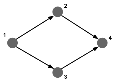
What if we want to find a complex pattern in a graph, such as loops, triangles, alternative paths, etc (see above)? Let’s say we want to find any alternative paths of length 3: where there are flights from airport 1 to airport 2 and from airport 2 to airport 4, but also from airport 1 to airport 3 and from airport 3 to airport 4.
Let’s check if there are alternative paths of length 2 between JFK and San Francisco SFO:
FOR v,e,p IN 2..2 ANY "airports/JFK" flights
FILTER v._id == 'airports/SFO'
LIMIT 5000
RETURN DISTINCT p.vertices[1]._id
It seems that there are many, including Atlanta (ATL), Boston (BOS), Phoenix (PHX), etc.
For an in-depth explanation on pattern matching, see here.
Centrality
As mentioned above, not all ArangoDB functonality is available through the web interface. For centrality queries and community detection, we’ll have to refer you to the arangosh documentation and community detection tutorial.
6.5 Improving performance of ArangoDB queries
As with any other database system, the actual setup of your database and how you write your query can have a huge impact on how fast the query runs.
Indices
Consider the following query which returns all flights of the plane with tail number “N937AT”.
FOR f IN flights
FILTER f.TailNum == 'N937AT'
RETURN f
This takes more than 3 seconds to run. If we explain this query (click the “Explain” button instead of “Execute”), we see the following:
Query String:
 FOR f IN flights
 FILTER f.TailNum == 'N937AT'
 RETURN f

Execution plan:
 Id   NodeType                    Est.   Comment
  1   SingletonNode                  1   * ROOT
  2   EnumerateCollectionNode   286463     - FOR f IN flights   /* full collection scan */
  3   CalculationNode           286463       - LET #1 = (f.`TailNum` == "N937AT")   /* simple expression */   /* collections used: f : flights */
  4   FilterNode                286463       - FILTER #1
  5   ReturnNode                286463       - RETURN f

Indexes used:
 none

Optimization rules applied:
 none
We see that the query loops over all 286463 documents and checks for each if its TailNum is equal to N937AT. This is very expensive, as a profile (Click the “Profile” button) also shows:
Query String:
 FOR f IN flights
 FILTER f.TailNum == 'N937AT'
 RETURN f

Execution plan:
 Id   NodeType                  Calls    Items   Runtime [s]   Comment
  1   SingletonNode                 1        1       0.00000   * ROOT
  2   EnumerateCollectionNode     287   286463       1.03926     - FOR f IN flights   /* full collection scan */
  3   CalculationNode             287   286463       0.10772       - LET #1 = (f.`TailNum` == "N937AT")   /* simple expression */   /* collections used: f : flights */
  4   FilterNode                    1       86       0.17727       - FILTER #1
  5   ReturnNode                    1       86       0.00000       - RETURN f

Indexes used:
 none

Optimization rules applied:
 none

Query Statistics:
 Writes Exec   Writes Ign   Scan Full   Scan Index   Filtered   Exec Time [s]
           0            0      286463            0     286377         1.32650

Query Profile:
 Query Stage           Duration [s]
 initializing               0.00000
 parsing                    0.00012
 optimizing ast             0.00000
 loading collections        0.00001
 instantiating plan         0.00007
 optimizing plan            0.00106
 executing                  1.32438
 finalizing                 0.00050
What we should do here, is create an index on TailNum. This will allow the system to pick those documents that match a certain tail number from a hash rather than having to check every single document. To create an index, go to Collections, and click on the flights collection. At the top you’ll see Indexes.
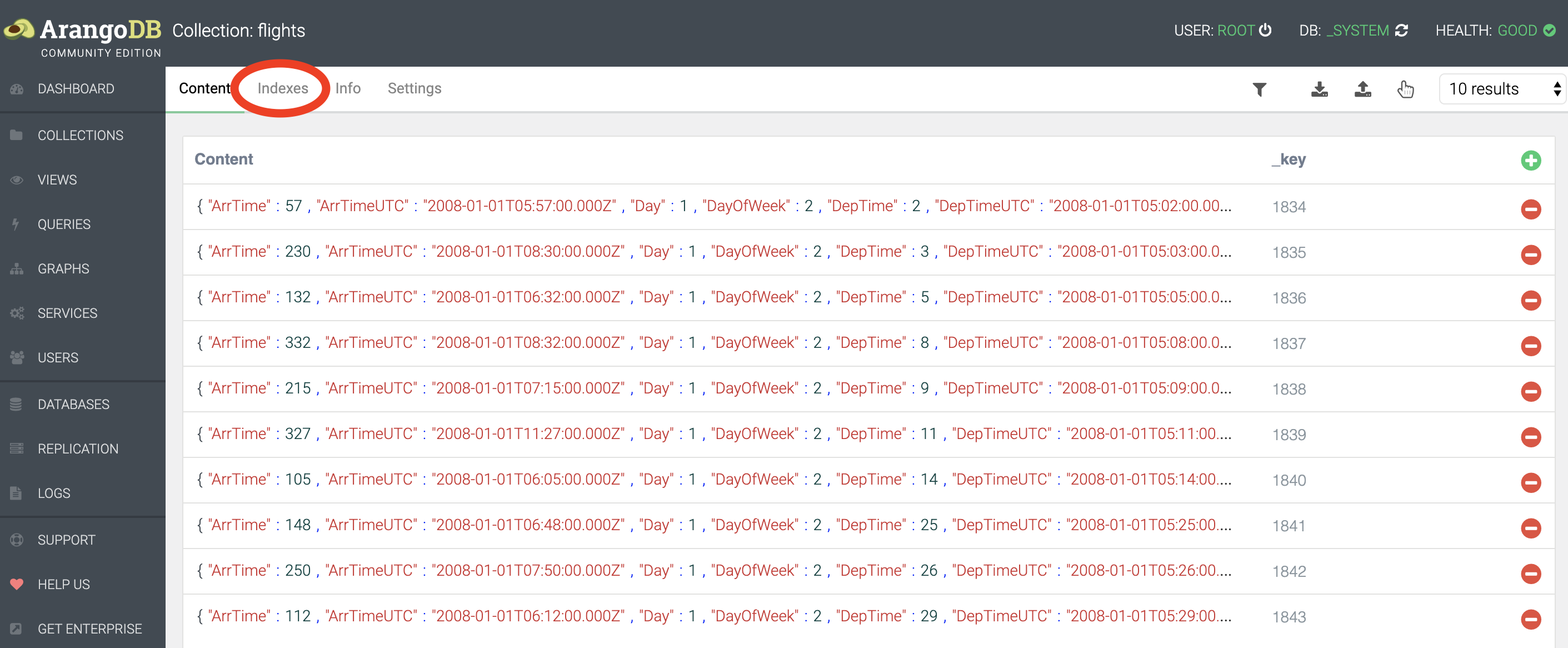
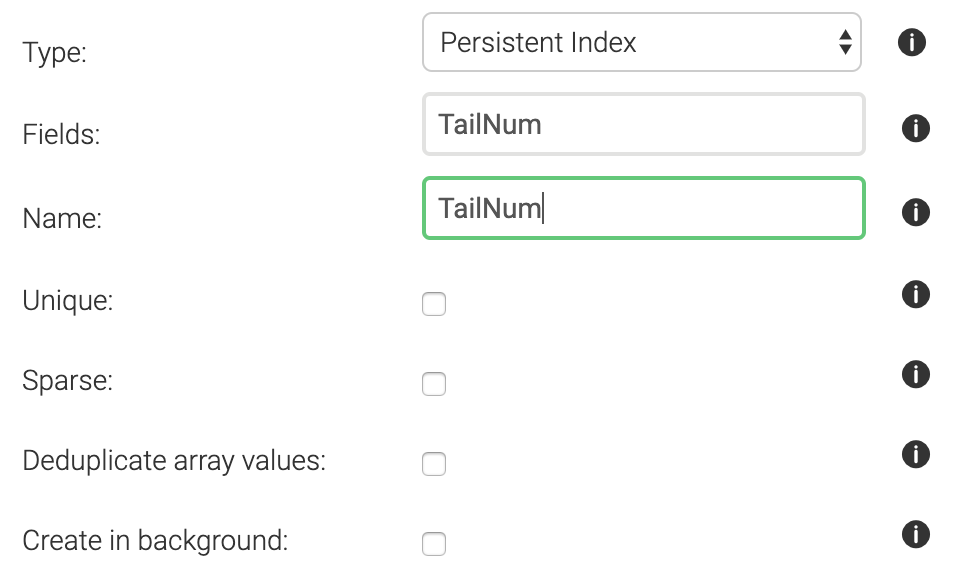
We’ll want to create a persistent index with the following settings (i.e. tail number is not unique across all flights, and is not sparse (in other words: tail number is almost always provided)):
After creating the index, an explain shows that we are not doing a full collection scan anymore:
Query String:
 FOR f IN flights
 FILTER f.TailNum == 'N937AT'
 RETURN f

Execution plan:
 Id   NodeType        Est.   Comment
  1   SingletonNode      1   * ROOT
  6   IndexNode         60     - FOR f IN flights   /* persistent index scan */
  5   ReturnNode        60       - RETURN f

Indexes used:
 By   Name      Type         Collection   Unique   Sparse   Selectivity   Fields          Ranges
  6   TailNum   persistent   flights      false    false         1.66 %   [ `TailNum` ]   (f.`TailNum` == "N937AT")

Optimization rules applied:
 Id   RuleName
  1   use-indexes
  2   remove-filter-covered-by-index
  3   remove-unnecessary-calculations-2
And indeed, running profile gives consistent results:
Query String:
 FOR f IN flights
 FILTER f.TailNum == 'N937AT'
 RETURN f

Execution plan:
 Id   NodeType        Calls   Items   Runtime [s]   Comment
  1   SingletonNode       1       1       0.00000   * ROOT
  6   IndexNode           1      86       0.00282     - FOR f IN flights   /* persistent index scan */
  5   ReturnNode          1      86       0.00000       - RETURN f

Indexes used:
 By   Name      Type         Collection   Unique   Sparse   Selectivity   Fields          Ranges
  6   TailNum   persistent   flights      false    false         1.66 %   [ `TailNum` ]   (f.`TailNum` == "N937AT")

Optimization rules applied:
 Id   RuleName
  1   use-indexes
  2   remove-filter-covered-by-index
  3   remove-unnecessary-calculations-2

Query Statistics:
 Writes Exec   Writes Ign   Scan Full   Scan Index   Filtered   Exec Time [s]
           0            0           0           86          0         0.00327

Query Profile:
 Query Stage           Duration [s]
 initializing               0.00000
 parsing                    0.00009
 optimizing ast             0.00001
 loading collections        0.00001
 instantiating plan         0.00003
 optimizing plan            0.00016
 executing                  0.00287
 finalizing                 0.00009
With the index, our query is 406 times faster. Instead of going over all 286463 documents in the original version, now it only checks 86.
Avoid going over supernodes
(Note: the following is largely based on the white paper “Switching from Relational Databases to ArangoDB” available at https://www.arangodb.com/arangodb-white-papers/white-paper-switching-relational-database/)
Super nodes are nodes in a graph with very high connectivity. Queries that touch those nodes will have to follow all those edges. Consider a database with songs information that is modelled like this:
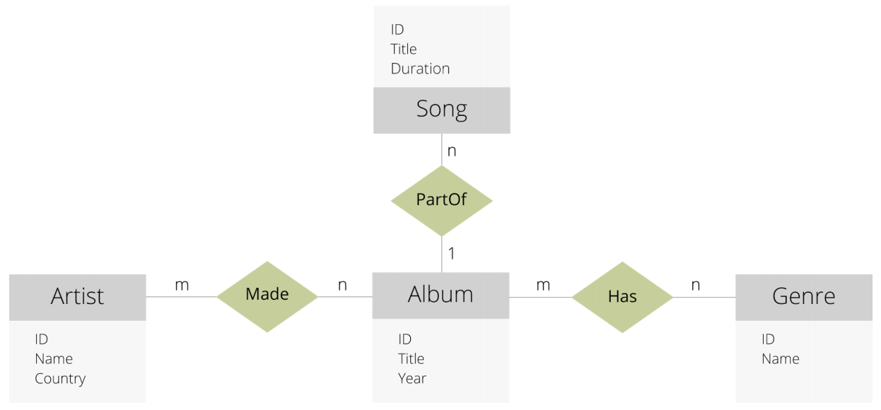
Source: White paper mentioned above
There are 4 document collections (Song, Artist, Album and Genre), and 3 edge collections (Made, PartOf and Has).
Some of Aerosmith’s data might look like this:
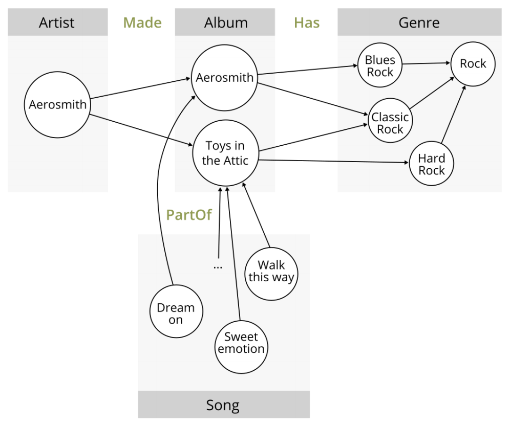
Source: White paper mentioned above
Suppose that we want to answer this question: ““I just listened to a song called, Tribute and I liked it very much. I suspect that there may be other songs of the same genre as this song that I might enjoy. So, I want to find all of the albums of the same genre that were released in the same year”. Here’s a first stab at such query.
Version 1:
FOR s IN Song
  FILTER s.Title == "Tribute"
  // We want to find a Song called Tribute
    FOR album IN 1 INBOUND s PartOf
    // Now we have the Album this Song is released on
      FOR genre IN 1 OUTBOUND album Has
      // Now we have the genre of this Album
        FOR otherAlbum IN 1 INBOUND genre Has
        // All other Albums with this genre
          FILTER otherAlbum.year == album.year
          // Only keep those where the year is identical
            RETURN otherAlbum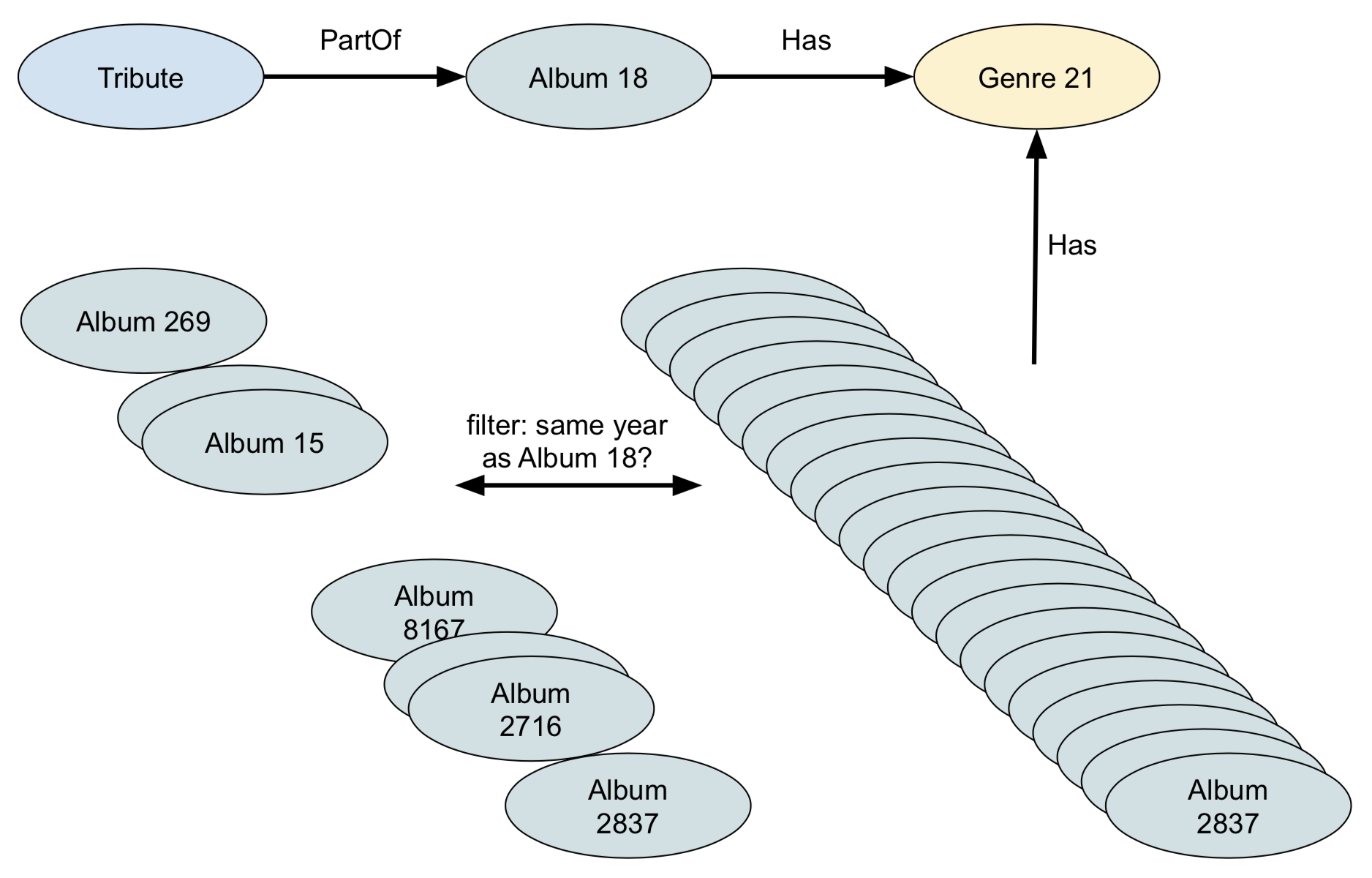
All goes well until we hit FOR otherAlbum IN 1 INBOUND genre Has, because at that point it will follow all links to the albums of that genre. It’s therefore better to first select all albums of the same year, and filter for the genre. This way we’ll only get a limited number of albums, and each of them has only one genre.
Version 2:
FOR s IN Song
  FILTER s.Title == "Tribute"
  // We want to find a Song called Tribute
    FOR album IN 1 INBOUND s PartOf
    // Now we have the Album this Song is released on
      FOR genre IN 1 OUTBOUND album Has
      // Get the genres of this Album
        FOR otherAlbum IN Album
        // Now we want all other Albums of the same year
          FILTER otherAlbum.Year == album.Year
          // So here we join album with album based on identical year
            FOR otherGenre IN 1 OUTBOUND otherAlbum Has
              FILTER otherGenre == genre
              // Validate that the genre of the other album is identical
              // to the genre of the original album
                RETURN otherAlbum
                // Finally return all albums of the same year
                // with the same genre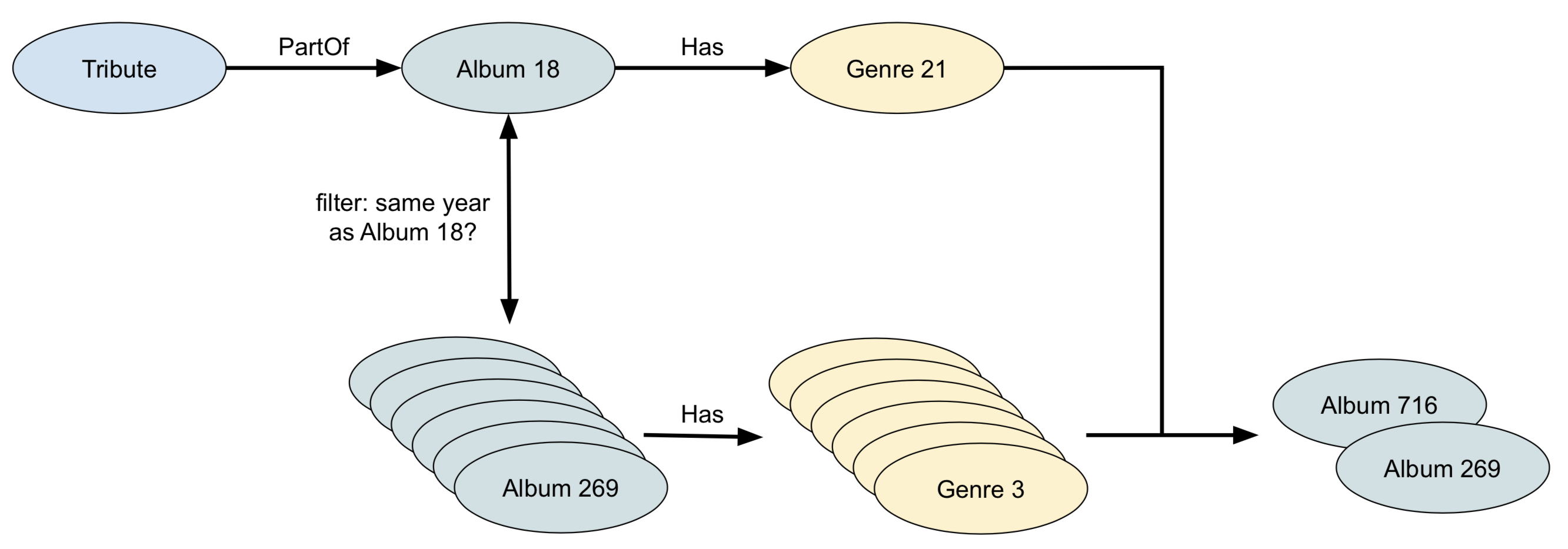
Again, a look at explain helps a lot here.
7. Using ArangoDB from R
You’ll often jump straight into the web interface or arangosh to do quick searches, but you will eventually also want to access that data from you analysis software, i.c. R. Most database systems have drivers for R, including ArangoDB: see here. The same is true for python (multiple libraries even, including ArangoPy and python-arango) and javascript, for example.
See the links for documentation on how to use ArangoDB from R and other languages. Just as an illustration: here’s a document query in R:
all.cities <- cities %>% all_documents()
all.persons <- persons %>% all_documents()
if(all.cities$London$getValues()$capital){
print("London is still the capital of UK")
} else {
print("What's happening there???")
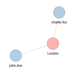
}And a graph query:
london.residence <- residenceGraph %>%
  traversal(vertices = c(all.cities$London), depth = 2)
london.residence %>% visualize()
will return: