The Lambda Architecture - how to handle huge and complex data
This post is part of the course material for the Software and Data Management course at UHasselt. The contents of this post is licensed as CC-BY: feel free to copy/remix/tweak/… it, but please credit your source.

- Part 1: Relational database design and SQL
- Part 2: Beyond SQL
- Part 3 (this post): Lambda Architecture
For a particular year’s practicalities, see http://vda-lab.be/teaching
Table of contents
In this post, we’ll revisit some of the more conceptual differences between using SQL and NoSQL databases, and touch upon the lambda architecture, which is a model to help you think about working with large and/or complex datasets.
Input for this post comes for a large part from the book by Marz and Warren “Big Data: Principles and best practices of scalable realtime data systems” (Manning Publications, 2015).
Note: whenever I mention “application” below, I’m not necessarily talking about a program complete with user interface that you can install on your Windows machine as a .exe or something that ends up in your Applications folder if you’re using OSX. “Application” is more generic than this, and also covers cases where you’re investigating data in R or SAS (either in an interactive or non-interactive way).
SQL vs NoSQL
As mentioned in the previous post, NoSQL is not about not using SQL, but about picking the right combination of database architectures.
We’ve seen that NoSQL is about a set of concepts that allow the rapid and efficient processing of datasets with a focus on performance, reliability and agility. Core themes are that these solutions:
- are free of joins
- are schema-free
- work on many processors
- can use shared-nothing commodity computers
- support linear scalability
To clarify this a bit more, we’ll dig a bit deeper into some of the central NoSQL concepts again.
Keep components simple
NoSQL systems are often created by integrating a number of modular functions that work together, in contrast to traditional RDBMS which are typically more integrated (mammoth) systems. Such simple components are set up in such way that they can be easily combined. You can compare this to the (very clever) linux pipeline system. When working on the linux command line, even knowing only a very limited number of commands you can do very complex things by piping these commands together: the output of one command becomes the input of the next.
Consider, for example,
cat data.csv | grep "chr1" | cut -f 2 | sort | uniq -c
This pipeline takes all data from the file data.csv, only keeps the lines that contain chr1, takes the second column, sorts this column, and returns the unique entries and how many there are for each. The same could have been done with a single script that we’d call count_of_unique_entries_in_column_2_for_chr1_in_datacsv.py. But by combining a set of commands that each only address part of the problem we can be much more agile, and it’s much easier to debug as well.
I like to think of NoSQL systems in a similar way: instead of using a single complex application, you glue together multiple simple components. In an application we wrote several years ago for clinical geneticists, we kept most data about patients, mutations and genes in a relational database. However, we also needed to access conservation scores across the genome. Basically this means that for every 3.1 billion bases in the genome we had 3 values. There is no way you’d use a relational database with 3x3.1 billion records in a table… For that we used a key/value store which is very good at this. This illustrates that in a NoSQL setting you look at what is necessary, and combine components that are good at solving parts of the problem. You can combine these afterwards in your application layer.
Use different application tiers
This is closely related to the lambda architecture that we’ll dig into further below.
Splitting up functionality in different tiers helps a lot to simplify the design of your application. By segregating an application into tiers you have the option of modifying or adding a specific layer instead of reworking an entire application, leading to a separation of concerns. The lambda architecture is a prime example of this. Also consider an application with a graphical user interface, which consists of a database layer, a computational layer which converts the raw data in the database to something that can be displayed, and the graphical user interface.
An important question to answer here is where to put the functionality of your application? In the last example: do you let the database compute (with e.g. SQL statements) the things you need in the graphical interface directly? Do you let the graphical user interface get the raw data from the database and do all the necessary munging of that data at the user end? Or do you insert a separate layer in between (i.e. the computational layer mentioned above)? It’s all about a separation of concerns.
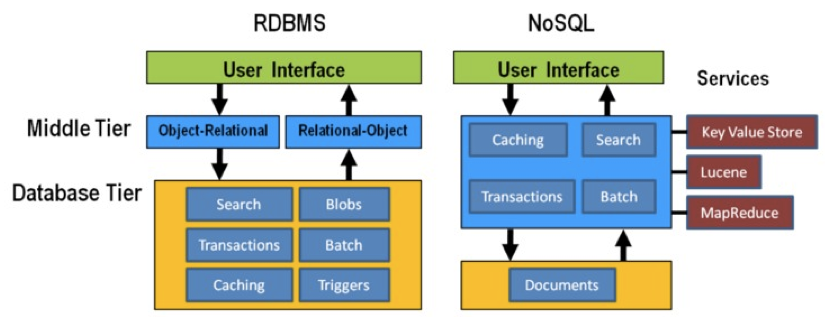
In general, RDBMS have been around for a long time and are very mature. As a result, a lot of functionality has been added to the database tier. In applications using NoSQL solutions, however, much of the application functionality is in a middle tier.
Think strategically about RAM, SSD and disk
To make sure that the performance of your application is adequate for your purpose, you have to think about where to store your data. Data can be kept in RAM, on a solid-state drive (SSD), the hard disk in your computer, or in a file somewhere on the network. This choice has an immense effect on performance. It’s easy to visualise this: consider that you are in Hasselt
- getting something from RAM = getting it from your backyard
- getting something from SSD = getting it from somewhere in your neighbourhood
- getting something from disk = traveling to Saudi Arabia to get it
- getting something over the network = traveling to Jupiter to get it
It might be clear to you that cleverly keeping things in RAM is a good way to speed up your application or analysis :-) Which brings us to the next point:
Keep your cache current using consistent hashing
So keeping things in RAM makes it possible to very quickly access them. This is what you do when you load data into a variable in your python/R/SAS/ruby/perl/… code.
Caching is used constantly by the computer you’re using at this moment as well.
An important aspect of caching is calculating a key that can be used to retrieve the data (remember key/value stores?). This can for example be done by calculating a checksum, which looks at each byte of a document and returns a long sequence of letters and numbers. Different algorithms exists for this, such as MD5 or SHA-1. Changing a single bit in a file (this file can be binary or not) will completely change the checksum.
Let’s for example look at the checksum for the file that I’m writing right now. Here are the commands and output to get the MD5 and SHA-1 checksums for this file:
janaerts$ md5 2019-10-31-lambda-architecture.md
MD5 (2019-10-31-lambda-architecture.md) = a271e75efb769d5c47a6f2d040e811f4
janaerts$ shasum 2019-10-31-lambda-architecture.md
2ae358f1ac32cb9ce2081b54efc27dcc83b8c945  2019-10-31-lambda-architecture.md
As you can see, these are quite long strings and MD5 and SHA-1 are indeed two different algorithms to create a checksum. The moment that I wrote the “A” (of “As you can see”) at the beginning of this paragraph, the checksum changed completely. Actually, below are the checksums after adding that single “A”. Clearly, the checksums are completely different.
janaerts$ md5 2019-10-31-lambda-architecture.md
MD5 (2019-10-31-lambda-architecture.md) = b597d18879c46c8838ad2085d2c7d2f9
janaerts$ shasum 2019-10-31-lambda-architecture.md
45c5a96dd506b884866e00ba9227080a1afd6afc  2019-10-31-lambda-architecture.md
This consistent hashing can for example also be used to assign documents to specific database nodes.
In principle, it is possible that 2 different documents have the same hash value. This is called hash collision. Don’t worry about it too much, though. The MD5 algorithm generates a 128 bit string, which occurs once every 10^38 documents. If you generate a billion documents per second it would take 10 trillion times the age of the universe for a single accidental collision to occur…
Of course a group of researchers at Google tried to break this, and they were actually successful on February 23th 2017.
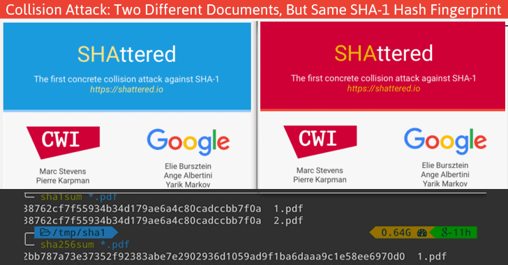
To give you an idea of how difficult this is:
- it had taken them 2 years of research
- they performed 9,223,372,036,854,775,808 (9 quintillion) compressions
- they used 6,500 years of CPU computation time for phase 1
- they used 110 years of CPU computation time for phase 2
ACID and BASE
ACID
RDBMS systems try to follow the ACID model for reliable database transactions. ACID stands for atomicity, consistency, isolation and durability. The prototypical example of a database that needs to comply to the ACID rules is one which handles bank transactions.
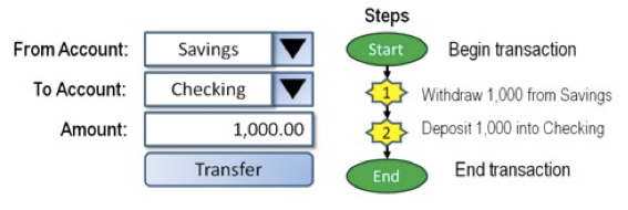
- Atomicity: Exchange of funds in example must happen as an all-or-nothing transaction
- Consistency: Your database should never generate a report that shows a withdrawal from saving without the corresponding addition to the checking account. In other words: all reporting needs to be blocked during atomic operations.
- Isolation: Each part of the transaction occurs without knowledge of any other transaction
- Durability: Once all aspects of transaction are complete, it’s permanent.
For a bank transaction it is crucial that either all processes (withdraw and deposit) are performed or none.
The software to handle these rules is very complex. In some cases, 50-60% of the codebase for a database can be spent on enforcement of these rules. For this reason, newer databases often do not support database-level transaction management in their first release.
As a ground rule, you can consider ACID pessimistic systems that focus on consistency and integrity of data above all other considerations (e.g. temporarily blocking reporting mechanisms is a reasonable compromise to ensure systems return reliable and accurate information).
BASE
BASE stands for:
- Basic Availability: Information and service capability are “basically available” (e.g. you can always generate a report).
- Soft-state: Some inaccuracy is temporarily allowed and data may change while being used to reduce the amount of consumed resources.
- Eventual consistency: Eventually, when all service logic is executed, the systems is left in a consistent state.
A good example of a BASE-type system is a database that handles shopping carts in an online store. It is no problem fs the back-end reports are inconsistent for a few minutes (e.g. the total number of items sold is a bit off); it’s much more important that the customer can actually purchase things.
This means that BASE systems are basically optimistic as all parts of the system will eventually catch up and be consistent. BASE systems therefore tend to be much simpler and faster as they don’t have to deal with locking and unlocking resources.
The Lambda Architecture
When working with large, complex or continuously changing data (aka “Big Data”), no single tool can provide a complete solution. In a big data situation, often a variety of tools and techniques is used. The Lambda Architecture helps us to organise everything. It decomposes the problem of computing arbitrary functions on arbitrary data in real-time by decomposing it into 3 layers:
- batch layer (least complex)
- serving layer
- speed layer (most complex)
Here’s the general picture:
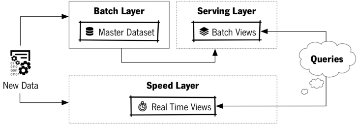
Lambda Architecture diagram (Costa & Santos, IAENG International Journal of Computer Science, 2017)
Let’s go through this figure layer by layer.
Batch layer
The batch layer needs to be able to (1) store an immutable, constantly growing master dataset, and (2) compute arbitrary functions on that dataset. You might sometimes hear the term “data lake”, which refers to a similar concept.
Immutable data storage
What does “immutable” mean? This data is never updated, only added upon. In SQL databases, you can update records like this (suppose that John Doe moved from California to New York):
UPDATE individuals
SET address = "302 Fairway Place",
    city = "Cold Spring Harbor",
    state = 'NY'
WHERE first_name = 'John'
AND last_name = 'Doe';
What this does is change the address in the database; the previous address in California is lost. In other words, the data is “mutated”.
Before the update:
| first_name | last_name | address | city | state |
|---|---|---|---|---|
| … | … | … | … | … |
| John | Doe | 101 Lake Avenue | Chowchilla | CA |
| … | … | … | … | … |
After the update:
| first_name | last_name | address | city | state |
|---|---|---|---|---|
| … | … | … | … | … |
| John | Doe | 302 Fairway Place | Cold Spring Harbor | NY |
| … | … | … | … | … |
In contrast, an immutable database would keep the original data as well; records can only be added, not changed. One way of doing this is to add timestamp to all records.
Let’s look at another example: friendships (which might change quicker or not than changes of address; that depends on the person…).
Instead of having a table with friendships, you record the data in a more raw form. For example:
| id | who | timestamp | action | to_who |
|---|---|---|---|---|
| 1 | Tom | 20100402 | add | Frank |
| 2 | Tony | 20100404 | add | Frank |
| 3 | Tom | 20100407 | remove | Frank |
| 4 | Tim | 20100409 | add | Frank |
| 5 | Tom | 20100602 | add | Freddy |
| 6 | Tony | 20100818 | add | Francis |
| 7 | Tony | 20101021 | add | Flint |
| 8 | Tony | 20110101 | add | Fletcher |
This is often called a facts table: the information in this table will always be true. Indeed, on June 2nd in 2010 Tom and Freddy became friends, whether or not they are still friends at this moment. Contrast that to the example above: John Doe will not always live at the address in California. Another way of thinking about this is that in the mutable version you record the state, whereas in the immutable version you record the changes to an underlying state.
As an exercise, what would an immutable version of the address example look like?
In these examples we’re adding records to a table, but the lambda layer can be implemented in many different ways. Rows can be added to a csv file; files can be added to a given directory; etc.
Everything starts with this immutable master dataset.
Computing arbitrary functions
Any query that we run is basically a function over the dataset: the query SELECT * FROM individuals WHERE name = "John Doe"; runs a filter function over the dataset in the individuals table. Looking at the above part on immutability, you might think “This is dumb. Just to find out who Tom’s friends are we have to go over the complete dataset and add/remove friends as we go.” Indeed, a table like the following would be much easier if you want to know how many friends everyone has (suppose you’re running the query on the first of November, 2019):
| id | who | nr_of_friends |
|---|---|---|
| 1 | Tom | 1 |
| 2 | Tony | 4 |
| 3 | Tim | 1 |
To know how many friends Tom has, the query would look like this:
SELECT nr_of_friends
FROM second_table
WHERE who = 'Tom';
Using the first table, it would have been:
SELECT COUNT('x') FROM (
  SELECT to_who
  FROM first_table
  WHERE who = 'Tom'
  AND action = 'add'
  AND timestamp < 20191101
  MINUS
  SELECT to_who
  FROM first_table
  WHERE who = 'Tom'
  AND action = 'REMOVE'
  AND timestamp < 20191101 );
Clearly, you want to use the shorter version of the two. However, the smaller table does not allow you to get the actual list of friends, or to get the number of friends that Tom had on the 8th of April 2010. That’s what we mean with “the batch layer should be able to compute arbitrary functions”.
But wait… Does that mean that we have to write such a complex query every time we want to get data from the database? No. That’s where the serving layer comes in.
Serving layer
The serving layer contains one or more versions of the data in a form that we want for specific questions. Let’s look at the friends example from above. We want to keep the original data in the batch layer, but also want to have easier versions to work with. These versions are computed by the batch layer, and are made available in what is called the serving layer.
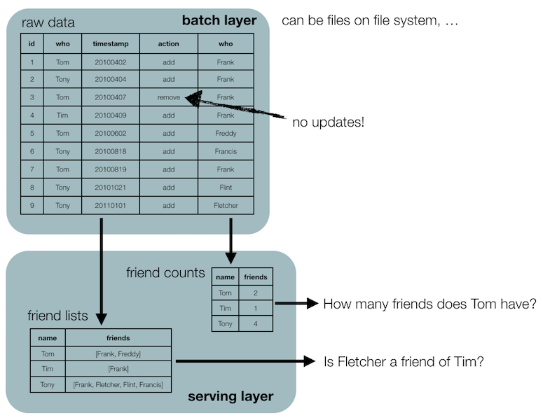
The “friend_counts” table, for example, can then be queried easily to get the number of friends for every individual. The serving layer therefore contains versions of the data optimised for answering specific questions.
This recomputation can be triggered by different things: it might start automatically when the previous round of recomputation has finished, it might start automatically whenever new data has been added, or (as in the example at the end of this post) it might be done on the fly when you’re for example using SQL views.
Making multiple views
Remember when we talked about data modeling in document-databases, that the way that the documents are embedded can have huge effects on performance. In our example there, genotypes could be organised by individual or by SNP.
{ name: "Tom",
  ethnicity: "African",
  genotypes: [
    { snp: "rs0001",
      genotype: "A/A",
      position: "1_8271" },
    { snp: "rs0002",
      genotype: "A/G",
      position: "1_127279" },
    { snp: "rs0003",
      genotype: "C/C",
      position: "1_82719" },
    ...
  ]}
{ name: "John",
  ethnicity: "Caucasian",
  ...
versus
{ snp: "rs0001",
  position: "1_8271",
  genotypes: [
    { name: "Tom",
      ethnicity: "African",
      genotype: "A/A" },
    { name: "John",
      ethnicity: "Caucasian",
      genotype: "A/A" },
    ...
  ]}
In a lambda architecture, if you know that you have to be able to answer both “what are the genotypes for a particular individual” and “what are the genotypes for a particular SNP” regularly, you’ll just create both versions of the data in the serving layer. You might think that this is dangerous because you might end up with inconsistencies when you have to update something. This was one of the reasons that we went for normalisation when we were talking about relational databases. There is however a big difference here: when we need to make a change, that change is added to the batch layer and would trickle down automatically to both versions in the serving layer.
Recomputation updates
The code necessary to create these “views” on the data is typically very simple. The batch layer continuously recomputes these views, which are then exposed in the serving layer (called batch views). These computations are conceptually very simple, because they always take all the data into consideration and basically delete the view and replace it with a completely new version. These are so-called recomputation updates, which are very different from incremental updates, in which the view remains where it is and only those parts that changed are updated. If the recomputation update is finished, it basically starts all over again.
Serving layer is out of date
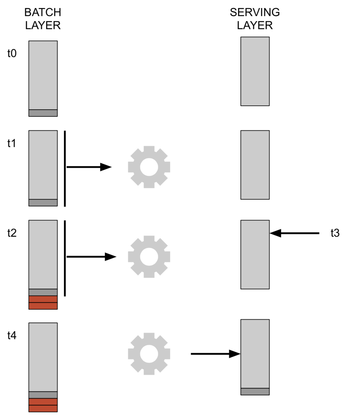
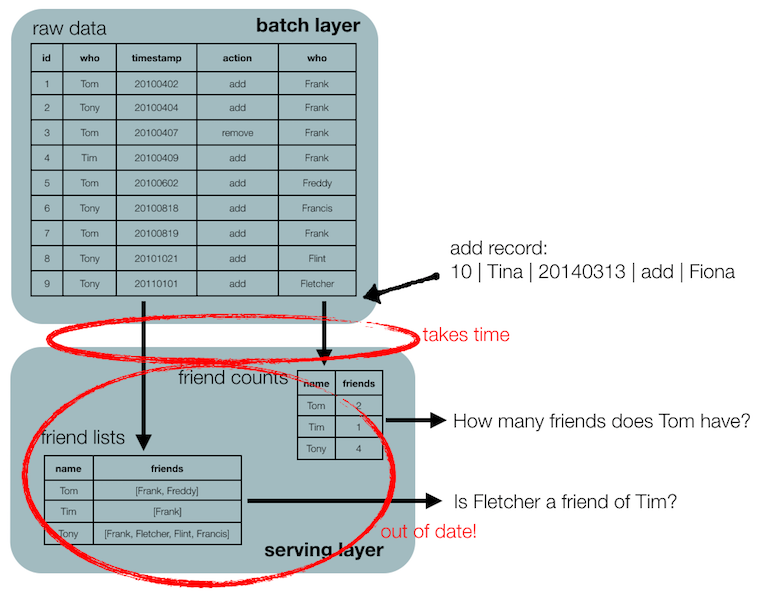
This approach does have a drawback, and that is that the data in the serving layer will always be out of date: the recomputation takes the data that is in the batch layer at the moment the computation begins, and does not look at any data that is added afterwards. Consider the image below. Let’s say that at timepoint t1 we have a serving layer and start its recomputation from the batch layer, and the recomputation is finished at t4. At timepoint t2 new data is added to the batch layer, but is not considered in the recomputation because that only took data into account that was in the batch layer at the start of the recomputation. At t3 we want to query the database (via the serving layer), and will miss the dark and the red datapoints because they are not in the serving layer yet. If we’d perform the same query at timepoint t4 we would include the dark grey datapoint.
Similarly, adding a record in the friends batch layer will take some time to become visible in the serving layer.
In many cases, having a serving layer that is slightly out of date is not really a problem. Think for example of the online store shopping cart mentioned above.
If it is really necessary to have the result of queries to be constantly up-to-date, we need a speed layer as well.
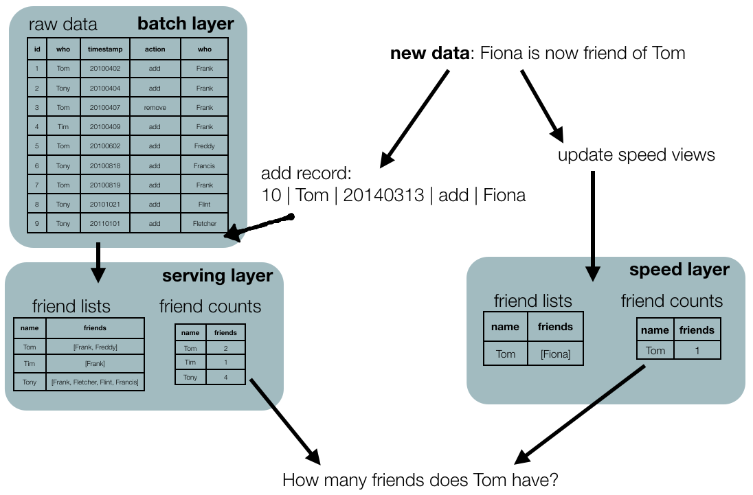
Speed layer
The answer to a question that we ask the serving layer will not include data that came in while the precomputation was running. The speed layer takes care of this. Similar to the batch layer, it creates a view of the data but those updates are incremental rather than a recomputation (see above). We won’t go into the speed layer too much because in most cases we can get away with not having one. If you don’t need a speed layer, don’t include it.
Only mentioning that:
- the speed layer is significantly more complex than the batch layer because updates are incremental
- the speed layer requires random reads and writes in the data while the batch layer only needs batch reads and writes
- the speed layer is only responsible for data that is not yet included in the serving layer, therefore the amount of data to be handled is vastly smaller
- the speed layer views are transient, and any errors are short-lived
An example
The batch layer master dataset can consist of files in a filesystem, records in some SQL tables, or any other way that we can store data. And although the lambda architecture is linked to the idea of Big Data and NoSQL, nothing prevents us from using a simple SQL database in this architecture if that fits our needs. Actually, the idea of views in a relational database corresponds to a serving layer, whereas the original tables in that case are the batch layer.
Consider the previous friends example.
CREATE VIEW v_nr_of_friends AS
SELECT COUNT('x') FROM (
  SELECT to_who
  FROM first_table
  WHERE action = 'add'
  AND timestamp < 20191101
  MINUS
  SELECT to_who
  FROM first_table
  WHERE action = 'remove'
  AND timestamp < 20191101 );
We have actually set up a local database to keep track of employee status and other information at the department. Although it is a relational database, it very much adheres to the lambda architecture paradigm. Here’s how (a very small part of) it is set up:
- Everything revolves around hiring contracts (i.e. information about when someone is hired, paid by which project, when the contract ends, etc). One person can have many consecutive contracts, for example when it’s a yearly contract that gets renewed.
- Information about the individual relates to their name, address, office number, work phone number, etc. Important: we do not remove an individual from this table when they leave the university.
- We compute a view v-current-individuals which - for each individual - checks if they have a current contract. This view therefore acts as the serving layer, as it is the one that we will actually query.
(For the way that the primary and foreign keys are set up in this example, see the normalisation explanation at /2019/08/extended-introduction-to-relational-databases).
contracts
| id | individual_id | start | end |
|---|---|---|---|
| 1 | 1 | 20170101 | 20171231 |
| 2 | 1 | 20180101 | 20181231 |
| 3 | 1 | 20190101 | 20191231 |
| 4 | 2 | 20170101 | 20171231 |
| 5 | 2 | 20180101 | 20181231 |
| 6 | 3 | 20190101 | 20191231 |
| 7 | 4 | 20160101 | 20161231 |
individuals
| id | name | office | phone number |
|---|---|---|---|
| 1 | Tom | A1 | 123-4567 |
| 2 | Tim | A9 | 123-5678 |
| 3 | Tony | A15 | 123-6789 |
| 4 | Tina | B3 | 123-7890 |
When someone new starts in the department, they are added to the individuals table; when someone gets a new contract, this is added to the contracts table (obviously a record is also created there when some is added to the individuals table because they’ll get their first contract at that moment…). Never is a record removed from either of these tables.
At the same time, we created an SQL view that computes the current individuals, i.e. those individuals that have a current contract. It looks something like this:
CREATE VIEW v_current_individuals AS
SELECT * FROM individuals i, contracts c
WHERE i.id = c.individual_id
AND c.start <= NOW()
AND c.end >= NOW();
A SELECT * FROM v_current_individuals therefore returns:
| id | name | office | phone number |
|---|---|---|---|
| 1 | Tom | A1 | 123-4567 |
| 3 | Tony | A15 | 123-6789 |
We could have set up the system in the regular way using updates, but we haven’t. If we had, the individuals table would have looked like this:
| id | name | office | phone number | end of contract |
|---|---|---|---|---|
| 1 | Tom | A1 | 123-4567 | 20191231 |
| 3 | Tony | A15 | 123-6789 | 20191231 |
Notice that Tim and Tina are not in this table, because they would have been removed. Similarly, when Tom would sign a new contract, the end of contract column would have been updated. But imagine that someone is erroneously removed from the individuals table: we can’t just add him or her again without finding out first what their address is, their office, etc. That data would have been lost
This example shows that in most real-life cases you want to have a mix of recomputation and updates, a mix between ACID and BASE. It’s almost never black-and-white: although we do not remove an individual from the individuals table when they leave (batch-layer approach), we do update an individual’s record when they change address, office, or phone number (non-lambda architecture approach).