Bi-Persistence Clustering on the Diabetes Dataset

In 1979, Reaven, Miller & Alto analysed the difference between chemical and overt diabetes in 145 non-obese adults. Previously, they had found a “horseshoe” relation between plasma glucose and insulin response levels, confirmed by later studies. However, the interpretation of this relationship remained unclear. It could be interpreted as the natural progression of diabetes or as different underlying causes for the disease. In their 1979 work, they attempted to quantify the relationship to gain insight into the pattern.

%load_ext autoreload
%autoreload 2

The autoreload extension is already loaded. To reload it, use:
  %reload_ext autoreload

import numpy as np
import pandas as pd

from umap import UMAP
from flasc import FLASC
from hdbscan import HDBSCAN
from biperscan import BPSCAN
from sklearn.preprocessing import StandardScaler

from lib.plotting import *
from matplotlib.colors import Normalize, to_rgb, ListedColormap
from matplotlib.lines import Line2D

tab10 = configure_matplotlib()

df = pd.read_csv("./data/diabetes/chemical_and_overt_diabetes.csv").iloc[:, 1:-1]
X = StandardScaler().fit_transform(df)

# X2 = UMAP(
#     n_neighbors=80, n_epochs=300, repulsion_strength=0.002, min_dist=0.1
# ).fit_transform(X)
# np.save("./data/diabetes/umap_embedding.npy", X2)

X2 = np.load("./data/diabetes/umap_embedding.npy")

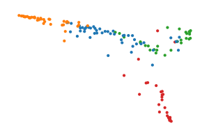
The dataset is projected to 2D using UMAP tuned to have a low repulsions strength and capture a lot of the global structure by considering a large number of neighbors. Datapoints are colored by the area under their glucose curve in red and the area under their insulin area in blue. The peaks of both features correspond to branches in the cluster’s shape:

glucose_norm = Normalize(df[" glucose area"].min(), df[" glucose area"].max())
glucose_colors = [
    (*to_rgb(plt.cm.Reds(glucose_norm(x))), glucose_norm(x))
    for x in df[" glucose area"]
]
insulin_norm = Normalize(df[" insulin area"].min(), df[" insulin area"].max())
insulin_colors = [
    (*to_rgb(plt.cm.Blues(insulin_norm(x))), insulin_norm(x))
    for x in df[" insulin area"]
]

sized_fig(0.33)
plt.scatter(*X2.T, s=1, color="silver")
plt.scatter(*X2.T, s=1, c=glucose_colors)
plt.scatter(*X2.T, s=1, c=insulin_colors)
plt.legend(
    loc="lower left",
    handles=[
        Line2D([0], [0], linewidth=0, marker=".", color="r", label="AUCG"),
        Line2D([0], [0], linewidth=0, marker=".", color="b", label="AUCI"),
    ],
)
plt.axis("off")
plt.subplots_adjust(0, 0, 1, 1)
plt.savefig("images/diabetes_umap.pdf", pad_inches=0)
plt.show()

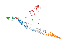
HDBSCAN struggles to detect these branches as distinct clusters. Only with the leaf cluster selection method and low min samples values will HDBSCAN detect small density peaks in the branches.

sized_fig(0.33)
c = HDBSCAN(min_cluster_size=5, cluster_selection_method="leaf").fit(X)
cmap = ListedColormap(["silver"] + [plt.cm.tab10.colors[i] for i in range(10)])
plt.scatter(*X2.T, c=c.labels_, s=1, cmap=cmap, vmin=-1, vmax=9)
plt.axis("off")
plt.subplots_adjust(0, 0, 1, 1)
plt.savefig("images/diabetes_hdbscan.pdf", pad_inches=0)
plt.show()

c:\Users\jelme\micromamba\envs\work\lib\site-packages\sklearn\utils\deprecation.py:151: FutureWarning: 'force_all_finite' was renamed to 'ensure_all_finite' in 1.6 and will be removed in 1.8.
  warnings.warn(
c:\Users\jelme\micromamba\envs\work\lib\site-packages\sklearn\utils\deprecation.py:151: FutureWarning: 'force_all_finite' was renamed to 'ensure_all_finite' in 1.6 and will be removed in 1.8.
  warnings.warn(

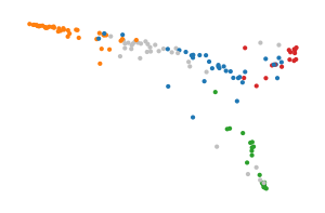
BPSCAN’s labels more closely match the projected shape (though, blue and green should be seen as a single cluster). The algorithm does require tuning: using low min samples values and a distance fraction up to 0.5 of the maximum distance grade.

sized_fig(0.33)
c = BPSCAN(min_samples=5, min_cluster_size=15).fit(X)
plt.scatter(*X2.T, c=c.labels_, s=1, cmap=cmap, vmin=-1, vmax=9)
plt.axis("off")
plt.subplots_adjust(0, 0, 1, 1)
plt.savefig("images/diabetes_bpscan.pdf", pad_inches=0)
plt.show()

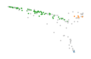
FLASC most accurately describes this dataset, as a single cluster with three branches. Most of the cluster is fairly central, indicated by the blue cluster. The other clusters indicate the branches, one of which is also very central and could be tuned out using a persistence threshold.

sized_fig(0.33)
c2 = FLASC(min_samples=5, min_branch_size=5, allow_single_cluster=True).fit(X)
plt.scatter(*X2.T, c=c2.labels_, s=1, cmap=cmap, vmin=-1, vmax=9)
plt.axis("off")
plt.subplots_adjust(0, 0, 1, 1)
plt.savefig("images/diabetes_flasc.pdf", pad_inches=0)
plt.show()

Additional Explanatory Figures

First, a plot showing Vietoris Rips complexes for merges in the centrality–distance space (use c.merge_hierarchy_ to find the merge ids to include in the plot).

c.merges_.plot_merges(*X2.T)

merge_ids = [2, 6, 15]
m = c.merges_
merges = m.merges
minpres = m.minpres
lens_values = [merges["lens_value"][i] for i in merge_ids]
distance_values = [merges["distance_value"][i] for i in merge_ids]
parent_sides = [merges["parent_side"][i] for i in merge_ids]
child_sides = [merges["child_side"][i] for i in merge_ids]
textcoords = [ (0.25, 0.5), (0.56, 0.5), (0.865, 0.5)]

import networkx as nx
from scipy.spatial.distance import squareform
from scipy.sparse import coo_array


def draw_vr_complex(x, y, dists, lens, dist_t, lens_t, xlim=None, ylim=None):
    # Extract edges within thresholds
    edges = coo_array(squareform(dists <= dist_t))
    edges.eliminate_zeros()
    g = nx.Graph(edges).subgraph(np.where(lens < lens_t)[0])
    node_list = [p for c in nx.connected_components(g) if len(c) > 1 for p in c]
    g = g.subgraph(node_list)

    # List triangular faces
    faces = []
    for source in g.nodes:
        for neighbor in g.neighbors(source):
            for second_degree in g.neighbors(neighbor):
                if source in g.neighbors(second_degree):
                    faces.append((source, neighbor, second_degree))
    poly = [
        [
            (x[face[0]], y[face[0]]),
            (x[face[1]], y[face[1]]),
            (x[face[2]], y[face[2]]),
        ]
        for face in faces
    ]

    # Prepare for plotting
    ax = plt.gca()
    pos = np.column_stack((x, y))
    node_list = list(g.nodes)
    edge_list = list(g.edges)
    node_colors = lens[node_list]

    # Draw points and edges
    mask = np.ones(len(x), dtype=bool)
    mask[node_list] = False
    plt.scatter(x[mask], y[mask], c="silver", s=3, edgecolors="none", linewidths=0)
    nx.draw_networkx(
        g,
        pos=pos,
        ax=ax,
        edgelist=edge_list,
        nodelist=node_list,
        edge_color="k",
        node_color=node_colors,
        width=0.5,
        node_size=1,
        with_labels=False,
        cmap="viridis",
        vmin=0,
        vmax=1,
    )

    # Draw faces
    for face in range(len(faces)):
        p = plt.Polygon(poly[face], fc="k", alpha=0.015)
        ax.add_patch(p)

    if xlim is None:
        ax.set_aspect("equal")
        xlim = plt.xlim()
        ylim = plt.ylim()
    else:
        plt.xlim(xlim)
        plt.ylim(ylim)

fig = sized_fig(1, aspect=0.33)

# Draw minpres edges
plt.scatter(
    minpres["lens_value"],
    minpres["distance_value"],
    c="silver",
    s=1,
    edgecolors="none",
    linewidths=0,
)

# Draw merges
plt.scatter(
    lens_values, distance_values, c="black", s=6, edgecolors="white", linewidths=0.3
)

# Draw arrows
for i, txt in enumerate(merge_ids):
    plt.annotate(
        "",
        (lens_values[i], distance_values[i]),
        textcoords[i],
        textcoords=fig.transFigure,
        va="center",
        ha="center",
        arrowprops=dict(arrowstyle="->", color="black"),
    )

# Set outer axis labels
plt.ylabel("Distance ($d_{mreach}$)")
plt.xlabel("Centrality ($c$)")

# Draw VR complexes as overlapping subplots
labels = ["(a)", "(b)", "(c)"]
for i, txt in enumerate(merge_ids):
    row = i + 1
    plt.sca(fig.add_subplot(3, 3, (row, row+3), label=i))
    draw_vr_complex(
        *X2.T, c.distances_, c.lens_values_, distance_values[i], lens_values[i]
    )
    plt.gca().spines["top"].set_visible(True)
    plt.gca().spines["right"].set_visible(True)
    plt.gca().spines["bottom"].set_visible(True)
    plt.gca().spines["left"].set_visible(True)
    plt.xticks([])
    plt.yticks([])
    plt.xlabel(labels[i], labelpad=-10)

plt.subplots_adjust(0.07, 0.23, 1, 0.99)
plt.savefig("images/diabetes_vr_complex.pdf", pad_inches=0)
plt.show()

Second, the minimal presentation edges as curves in the centrality–distance plane. Three curves are highlighted, corresponding to the low(est)-centrality points in the branches.

sized_fig()
minpres = c.minimal_presentation_
minpres.plot_persistence_areas(
    view_type="value", line_kws=dict(alpha=0.1, linestyle="-", linewidths=0.5)
)
plt.xlabel('Centrality')
plt.ylabel('Distance')
curves = minpres.compute_value_death_curves()
for i, p in enumerate([1, 13, 31]):
    plt.plot(*curves[p].T, color=f"C{i+1}", linewidth=1)
plt.subplots_adjust(0.13, 0.23, 1, 1)
plt.savefig("images/diabetes_minpres_values.pdf", pad_inches=0)
plt.show()

Third, the minimum presentation as a graph. Points are coloured by centrality grade and edges are coloured by distance grade. The three root points are indicated by crosses.

sized_fig()
pos = minpres.plot_network(
    layout={i: (c[0], c[1]) for i, c in enumerate(X2)},
    labels=False,
    node_kws=dict(node_size=5, edgecolors="none", linewidths=0),
    line_kws=dict(width=0.5, arrowsize=2, alpha=0.5, edge_vmin=-1000, edge_vmax=4000),
)
for i, p in enumerate([1, 13, 31]):
    plt.plot(*X2[c._row_to_point[p]].T, "x", color=f"C{i+1}", markersize=4)
plt.subplots_adjust(0, 0, 1.2, 1)
plt.savefig("images/diabetes_minpres_network.pdf", pad_inches=0)
plt.show()

Next, the merge hierarchy and its merges:

sized_fig(1, 0.33)
m.plot_persistence_areas(view_type='value')
plt.xlim(0.67, 0.93)
plt.xlabel('Centrality')
plt.ylabel('Distance')
plt.subplots_adjust(0.08, 0.22, 1.02, 0.97)
plt.savefig("images/diabetes_merge_hierarchy_values.pdf", pad_inches=0)
plt.show()

sized_fig(1, 0.618/4*3)
m.plot_merges(*X2.T, s=2, arrowsize=8, linewidth=0.5)
plt.subplots_adjust(0, 0, 1, 0.96, 0, 0)
plt.savefig("images/diabetes_merge_hierarchy_points.pdf", pad_inches=0)
plt.show()

Now, the simplified hierarchy and its merges:

sized_fig(1, 0.33)
c.simplified_merges_.plot_persistence_areas(view_type='value')
plt.xlim(0.67, 0.93)
plt.xlabel('Centrality')
plt.ylabel('Distance')
plt.subplots_adjust(0.08, 0.22, 1.02, 0.97)
plt.savefig("images/diabetes_simplified_hierarchy_values.pdf", pad_inches=0)
plt.show()

sized_fig(1, 0.618/2)
c.simplified_merges_.plot_merges(*X2.T, s=2, n_rows=1, n_cols=2)
plt.subplots_adjust(0, 0, 1, 0.96, 0, 0)
plt.savefig("images/diabetes_simplified_hierarchy_points.pdf", pad_inches=0)
plt.show()

Finally, the full linkage hierarchy in distance–centrality space and as a network.

h = c.linkage_hierarchy_

sized_fig()
h.plot_persistence_areas(
    view_type="value",
    node_kws=dict(s=1, edgecolors="none", linewidths=0),
    line_kws=dict(lw=0.2, color="silver"),
    labels=False,
)
plt.xlabel("Centrality")
plt.ylabel("Distance")
plt.subplots_adjust(0.13, 0.23, 1.22, 0.99)
plt.savefig('images/diabetes_linkage_hierarchy_values.pdf', pad_inches=0)
plt.show()

sized_fig()
pos = h.plot_network(
    layout="sfdp",
    node_kws=dict(node_size=0.4, edgecolors="none", linewidths=0),
    line_kws=dict(width=0.1, arrowsize=2, edge_vmin=-1000, edge_vmax=8000),
    labels=False,
)
# xs = [pos[i][0] for i in range(len(df))]
# ys = [pos[i][1] for i in range(len(df))]
# plt.scatter(xs, ys, c=c.labels_, s=1, cmap=cmap, vmin=-1, vmax=9)
plt.subplots_adjust(0, 0, 1.2, 1)
plt.savefig("images/diabetes_linkage_hierarchy_network.pdf", pad_inches=0)
plt.show()