How Lensed UMAP works

This notebook demonstrates three functions for filtering UMAP graphs to efficiently explore data from flexible perspective.

%load_ext autoreload
%autoreload 2

import numpy as np
import pandas as pd
import lensed_umap as lu
from umap import UMAP

from lib.plotting import *
configure_matplotlib()

import warnings
warnings.filterwarnings("ignore", lineno=151, module=r"sklearn.*")

Demonstration data

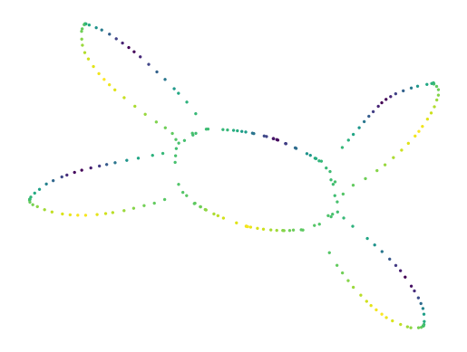
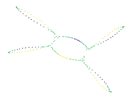
We use a simple dataset for this demonstration. Each point has a 2D position and an additional signal-value, shown below. The points form an interesting structure, with one loop and four flares sticking out. Each flare has a signal local minimum and maximum towards its center.

df = pd.read_csv("./data/five_circles.csv", header=0)
lens = np.log(df.hue)

sized_fig(1)
plt.scatter(df.x, df.y, 2, lens, cmap="viridis")
plt.axis("off")
plt.colorbar(label='signal')
plt.show()

Default UMAP

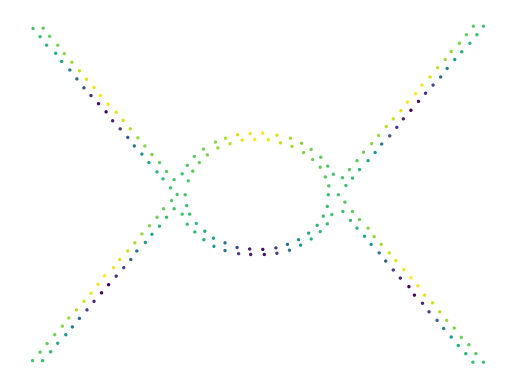
Exploration starts from a normal UMAP model. In some cases, time can be saved by only constructing UMAP’s graph and leaving computing the 2D layout for later. In this example, we reduce the repulsion strength in the 2D layout to ensure the loop remains intact. Otherwise, the process is quite normal.

projector = UMAP(
    repulsion_strength=0.1,  # To avoid tears in projection that
    negative_sample_rate=2,  # are not in the modelled graph!
).fit(df[["x", "y"]])
print(f"Constructed graph with {projector.graph_.size} edges")

sized_fig(1)
x, y = lu.extract_embedding(projector)
plt.scatter(x, y, 2, lens, cmap="viridis")
plt.axis("off")
plt.show()

Constructed graph with 3408 edges

Global Lens

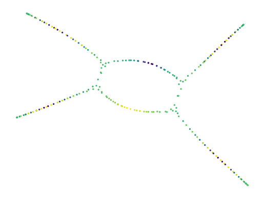
The first filter function is apply_lens. This function takes a fitted UMAP object and returns a (shallow) copy of that object with a new graph_ and embedding_ attributes. To apply the filter, the function discretizes the given 1D signal into segments. Then, the graph is filtered to keep only edges that cross at most one segment boundary. Finally, the layout is updated for the new graph.

The cell below demonstrates the function in action. Notice how the four flares became circles, separating the local extrema from each other.

lensed = lu.apply_lens(projector, lens, resolution=6, discretization="balanced")
print(f"Constructed graph with {lensed.graph_.size} edges")

sized_fig(1)
x, y = lu.extract_embedding(lensed)
plt.scatter(x, y, 2, lens, cmap="viridis")
plt.axis("off")
plt.show()

Constructed graph with 2202 edges

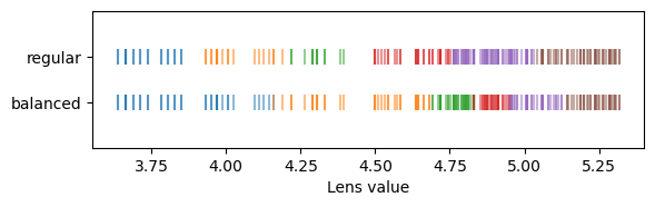
This function supports two kinds discretization strategies: regular and balanced.

• Regular is the default and creates equally sized segments. With regular segments, the filter reduces to a global filter-value-difference threshold that removes all edges with a filter-value-difference larger than the one segment width.

• Balanced creates segments that contain the same number of points (except the last one may be slightly larger than the others). As a consequence, the filter-value-difference threshold varies with the filter-distribution’s density: for uncommon filter-values the threshold is higher and for common filter-values the threshold is smaller.

def scatter_segments(projector, lens, y, strategy):
    colors = lu.apply_lens(
        projector,
        lens,
        resolution=6,
        discretization=strategy,
        skip_embedding=True,
        ret_bins=True,
    )[1]
    plt.scatter(
        lens,
        np.repeat(y, len(x)),
        100,
        colors,
        marker="|",
        alpha=0.5,
        cmap="tab10",
        vmin=0,
        vmax=10,
    )


sized_fig(1, 1/3)
scatter_segments(projector, lens, 1, "regular")
scatter_segments(projector, lens, 0, "balanced")
plt.xlabel("Lens value")
plt.ylim([-1, 2])
plt.yticks([0, 1])
plt.gca().set_yticklabels(["balanced", "regular"])
plt.show()

Global Mask

The second function is apply_mask. This function takes two UMAP models: projector and masker. Then, it creates a (shallow) copy of projector and updates the graph keeping only the edges that also exist in masker. This can be seen as an intersection, but the edges keep projector’s weights! Finally, the 2D layout is updated for the new graph. To save some compute cost, masker can be fitted with transform_mode="graph", which skips the 2D layout step.

Like the previous function, this strategy can be reduced to a varying filter-distance threshold. Here, that threshold is expressed as the number of neighbours to keep in the filter-dimensions. As a consequence, masker’s n_neighbor value may need to be quite big to avoid removing too many edges, which can be expensive to compute. Different from the global lens, this strategy is not limited to a 1D lens dimension. Instead it uses anything that UMAP accepts.

masker = UMAP(n_neighbors=150, transform_mode="graph").fit(df.hue.to_numpy()[None].T)
lensed = lu.apply_mask(projector, masker)
print(f"Constructed graph with {lensed.graph_.size} edges")

sized_fig(1)
x, y = lu.extract_embedding(lensed)
plt.scatter(x, y, 2, lens, cmap="viridis")
plt.axis("off")
plt.show()

Constructed graph with 2576 edges

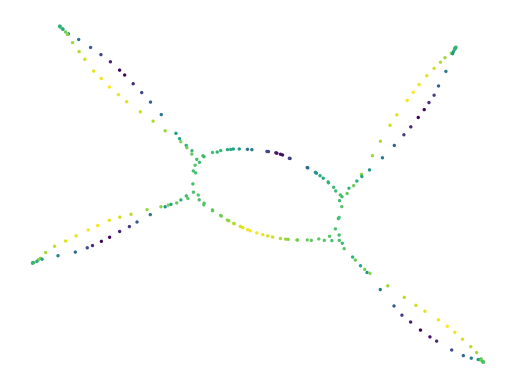
Local Mask

The last function is apply_local_mask. This function takes a UMAP model and returns a (shallow) copy with updated graph and 2D layout. The function first computes a distance in the filter dimensions for each UMAP model’s edge. Then, the closest n_neighbors edges are kept for each point (with ties broken by the edge’s strength). Like with the global mask, edges keep their initial weights. Finally, the 2D layout is updated.

This strategies does not reduce to a global threshold. Instead, the threshold varies with the spread of filter-values across the initial UMAP manifold.

This strategy’s parameters are quite intuitive. They directly specify how many edges to keep. The other strategies indirectly specify which edges to remove, which can be more difficult to reason about.

lensed = lu.apply_local_mask(projector, df.hue)
print(f"Constructed graph with {lensed.graph_.size} edges")

sized_fig(1)
x, y = lu.extract_embedding(lensed)
plt.scatter(x, y, 2, lens, cmap="viridis")
plt.axis("off")
plt.show()

Constructed graph with 1346 edges