Case Study: Air Quality

This notebook analyses the air-quality dataset collected by the Castile and León initiative in Spain, previously analysed by Alcaide & Aerts (2020). They found several interesting patterns that we attempt to re-discover using UMAP filters. The goal of this notebook is to demonstrate using the filtering functions to inspect different perspectives.

Setup

Loading libraries:

%load_ext autoreload
%autoreload 2

# Data
import re
import time
import warnings
import numpy as np
import numba as nb
import pandas as pd
from datetime import date
from anndata import AnnData
from anndata._core.anndata import ImplicitModificationWarning
from sklearn.impute import KNNImputer
from sklearn.preprocessing import RobustScaler
from sklearn.datasets import make_classification, make_blobs
from scipy.spatial.distance import cdist

# UMAP
from umap import UMAP
from umap.umap_ import reset_local_connectivity as reset_connectivity
import lensed_umap as lu
from fast_hdbscan import HDBSCAN

# Plotting
import datashader as ds
import datashader.transfer_functions as tf
from datashader.bundling import connect_edges
import matplotlib.pyplot as plt
from matplotlib.colors import to_hex
from matplotlib.lines import Line2D
from matplotlib.gridspec import GridSpecFromSubplotSpec
from lib.plotting import *

configure_matplotlib()
# Disable specific warnings to clean up the output
warnings.filterwarnings("ignore", lineno=151, module=r"sklearn.*")
warnings.filterwarnings("ignore", category=nb.core.errors.NumbaWarning)
warnings.filterwarnings("ignore", category=ImplicitModificationWarning)

The data

The data describes seven chemical’s concentration in the air (CO (mg/m3), NO (ug/m3), NO2 (ug/m3), SO2 (ug/m3), O3 (ug/m3), PM10 (ug/m3), PM25 (ug/m3)). Measurements are taken daily at several locations, with more locations being added over time. The measurements started in 1997 and ran till the end of 2020. We load the data from a .csv file and construct an AnnData object splitting features from metadata.

seasons = ["winter", "spring", "summer", "autumn"]
periods = ["1997-2002", "2003-2008", "2009-2014", "2015-2020"]
year_ticks = np.asarray([int(p.split("-")[0]) for p in periods])


def classify_year(year):
    """Returns the period for a given year."""
    idx = np.where(year < year_ticks)[0]
    idx = idx[0] if 0 < len(idx) else 0
    return periods[idx - 1]


def load_data():
    raw = (
        pd.read_csv("./data/air/calidad-del-aire-datos-historicos-diarios.csv", sep=";")
        .rename(
            columns={"Fecha": "date", "Latitud": "latitude", "Longitud": "longitude"}
        )
        .drop(columns=["Provincia", "Estación", "Posición"])
    )
    raw["year"] = raw.date.apply(lambda x: int(x.split("-")[0]))
    raw["month"] = raw.date.apply(lambda x: int(x.split("-")[1]))
    raw["day"] = raw.date.apply(lambda x: int(x.split("-")[2]))
    raw["week"] = raw.date.apply(
        lambda x: date(*[int(s) for s in x.split("-")]).isocalendar().week
    ).astype(int)
    raw["season"] = (
        raw.date.apply(lambda x: seasons[int(x.split("-")[1]) % 12 // 3])
        .astype("category")
        .cat.set_categories(seasons, ordered=True)
    )
    raw["period"] = (
        raw.year.apply(classify_year)
        .astype("category")
        .cat.set_categories(periods, ordered=True)
    )

    vdims = [col for col in raw.columns if " " in col]
    vdim_names = [col.split(" ")[0] for col in vdims]
    vdim_display_names = [
        re.sub(r"([^0-9])([0-9])$", r"\1$_\2$", col) for col in vdim_names
    ]
    units = [vdim.split(" ")[1].replace("(", "").replace(")", "") for vdim in vdims]
    andims = [
        "latitude",
        "longitude",
        "period",
        "year",
        "month",
        "day",
        "week",
        "season",
    ]

    raw.index = raw.index.astype(str)
    raw[vdims] = raw[vdims].mask(raw[vdims] < 0)
    df = AnnData(
        X=raw[vdims].rename(columns={v: name for v, name in zip(vdims, vdim_names)}),
        obs=raw[andims],
        var=pd.DataFrame.from_dict(
            dict(unit=units, name=vdim_display_names, index=vdim_names),
        ).set_index("index"),
    )
    return df


df = load_data()

The data contains numerous missing values. Alcaide & Aerts (2020) dealt with these missing values by aggregating measurements up to weeks. In this notebook, we take another approach, ensuring we keep locations separate and retain a larger number of observations. Specifically, we remove the columns with more than 40% missing values. Then, we remove observations with missing values in columns with more than 10% missing values. Finally, the remaining missing values are imputed using a KNNImputer. The concentrations are then scaled to be in the same value-range using a robust z-score. The resulting dataset contains 181.386 observations.

missing = pd.Series(np.isnan(df.X).sum(axis=0) / df.n_obs, index=df.var_names)
print(missing)

# Drop columns with more than 40% missing
df = df[:, ~df.var_names.isin(missing[missing > 0.4].index)]
# Drop observations with missing values in columns with more than 10%
df = df[~np.isnan(df[:, missing[df.var_names] > 0.1].X).any(axis=1), :]

# Impute missing values in columns with less than 10%
df.X = KNNImputer(n_neighbors=5, weights="distance").fit_transform(df.X)
df.X = RobustScaler().fit_transform(df.X)

index
CO      0.773195
NO      0.069475
NO2     0.072906
O3      0.382499
PM10    0.227426
PM25    0.879412
SO2     0.201290
dtype: float64

Custom code:

We use several functions throughout this notebook to simplify working with the data and UMAP models. The (hidden) cells in this section define those functions and constants.

• Colors for seasons, periods, and feature categories

Data processing:

• edge_paths transforms edges into a dataframe to efficiently plot them using datashader.

• melt_features pivots dataframe to treat features as categories when plotting.

• compute_projection computes and stores a UMAP projection in the AnnData frame.

• compute_lens computes and stores a lensed projection in the AnnData frame.

Datashader plotting with matplotlib:

• plot_points plots points coloured by a column in df.obs or df.X. Use the colorbar flag to switch between linear and eq_hist color-mapping. A manual clim is only supported in the colorbar mode.

• plot_category plots points coloured by a category column in df.obs or by each feature in df.X as a category. Requires a corresponding color mapping in df.uns['colors'].

• plot_edges creates and plots a line-segment dataframe with the edges in the given layout.

• plot_overview plots an overview with the highest feature, points coloured by year, and a small multiples with points coloured by feature.

Data exploration with filtered UMAP

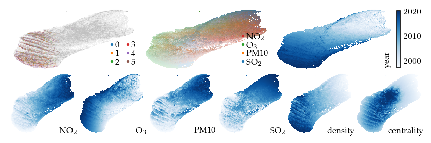
First, we compute density, centrality, and HDBSCAN* clusters which can serve as geometric filter dimension.

clusterer = HDBSCAN(min_samples=25, min_cluster_size=500).fit(df.X)

df.obs["density"] = 1 / (1 + clusterer._core_distances)
df.obs["centrality"] = 1 / (1 + cdist(np.average(df.X, axis=0)[None, :], df.X)[0])
df.obs["clusters"] = [f"{i}" for i in clusterer.labels_]
df.obs.clusters = df.obs.clusters.astype("category")
df.uns["colors"]["clusters"] = {"-1": to_hex("silver")}
df.uns["colors"]["clusters"].update(
    {f"{i}": to_hex(f"C{i%10}") for i in range(clusterer.labels_.max() + 1)}
)

Next, we compute the initial UMAP projection. This notebook uses cuML to accelerate computing UMAP layouts with Nvidia GPUs. If that is not available, change all lu.cuml_embed_graph function calls to lu.embed_graph. The latter function uses the UMAP package to compute layouts.

p = compute_projection(df, "default", n_neighbors=50)

Build UMAP model: 10.02s
Compute layout: 2.90s

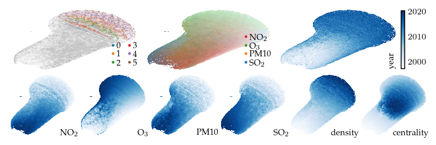
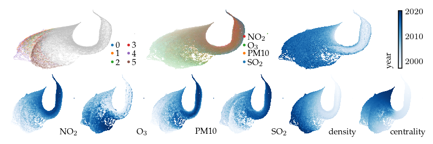
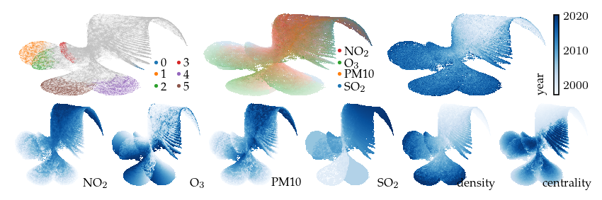
This projection is already quite interesting. The measurement year is strongly correlated with the embedding, even though it is not included as input. We also see that all density-based clusters contain only fairly recent measurements. The top-middle plot colors points by their highest (robust z-score normalized) feature, indicating which features have high values in different parts of the layout.

sized_fig(1, 0.618 / 3 + 0.618 / 6)
plot_overview(df, "default")
plt.show()

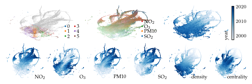
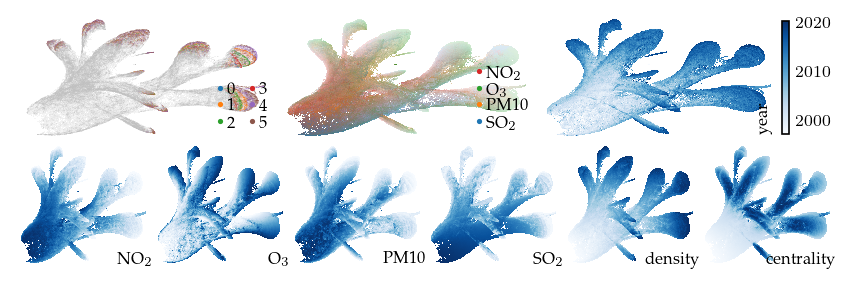
Now, lets explore the projection with filters. First, applying a filter on the measurement year dimension incorporates an additional signal in the embedding. This filter keeps only the edges between observations measured in the same or consecutive years. As a result, regions with similar features measured in different years are pulled apart. The branches (or flares) created by the filter indicate states that were not present for some of the years.

p_year = compute_lens(
    df,
    p,
    "year",
    fun=lu.apply_lens,
    values=df.obs["year"],
    resolution=((df.obs["year"].max() - df.obs["year"].min()) + 1),
    repulsion_strengths=[0.001, 0.01, 0.1, 1, 0.2],
)

Apply lens: 0.02s
Compute layout: 1.08s

sized_fig(1, 0.618 / 3 + 0.618 / 6)
plot_overview(df, "year")
plt.show()

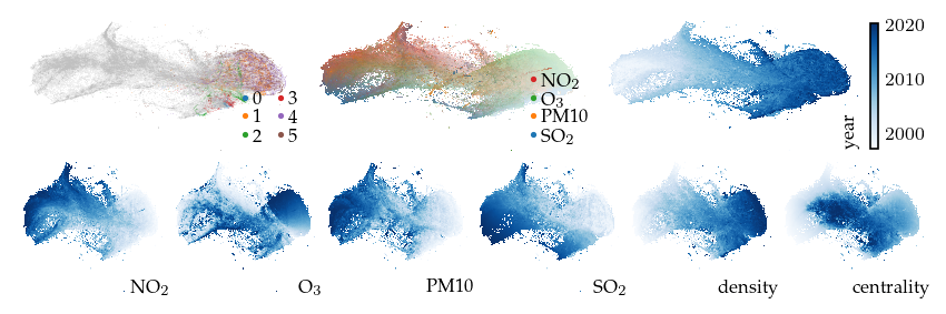
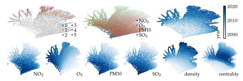
A filter emphasizing the SO2 feature creates an interesting perspective. The resulting embedding has slices that correspond to the density-based clusters and reveals discrete SO2 values.

p_sulfer = compute_lens(
    df,
    p,
    "sulfer",
    fun=lu.apply_local_mask,
    values=df[:, "SO2"].X,
    n_neighbors=20,
    repulsion_strengths=[0.001, 0.01, 0.1, 1, 0.2],
)

Apply lens: 1.06s
Compute layout: 1.42s

sized_fig(1, 0.618 / 3 + 0.618 / 6)
plot_overview(df, "sulfer")
plt.show()

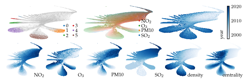
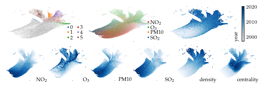
Applying a filter on the density signal is also interesting for exploring density based clusters. This filter 5 major density maxima and a single density minimum.

p_density = compute_lens(
    df,
    p,
    "density",
    fun=lu.apply_local_mask,
    values=df.obs["density"],
    n_neighbors=15,
    repulsion_strengths=[0.001, 0.01, 0.1, 1, 0.2],
)

Apply lens: 0.75s
Compute layout: 1.21s

sized_fig(1, 0.618 / 3 + 0.618 / 6)
plot_overview(df, "density")
plt.show()

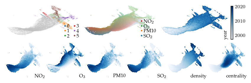
Applying a filter on centrality estimates can also provide interesting perspectives. Such filters can reveal low-density flares or branches. In this case, a centrality filter reveals one major centrality maxima (expected) and two centrality minima, indicating that there are no considerable flares.

p_centrality = compute_lens(
    df,
    p,
    "centrality",
    fun=lu.apply_local_mask,
    values=df.obs["centrality"],
    n_neighbors=15,
    repulsion_strengths=[0.001, 0.01, 0.1, 1, 0.2],
)

Apply lens: 0.82s
Compute layout: 1.24s

sized_fig(1, 0.618 / 3 + 0.618 / 6)
plot_overview(df, "centrality")
plt.show()

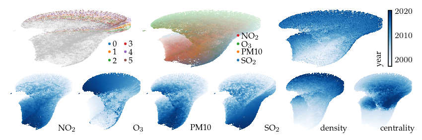
Filters can also be used to incorporate features that inherently use different notions of distance. For example, a filter on GPS coordinates using the haversine distance. This filter separates similar observations by their measurement location. The resulting embedding appears to have several ‘strands’ for early measurements, while more recent measurements remain connected.

p_gps = compute_lens(
    df,
    p,
    "gps",
    fun=lu.apply_local_mask,
    values=df.obs[["latitude", "longitude"]],
    metric="haversine",
    n_neighbors=5,
    reset_local_connectivity=True,
    repulsion_strengths=[0.001, 0.01, 0.1, 1, 1, 0.1, 0.1],
)

Apply lens: 1.12s
Compute layout: 0.82s

sized_fig(1, 0.618 / 3 + 0.618 / 6)
plot_overview(df, "gps")
plt.show()

Finally, emphasizing the Ozon feature with a filter separates the density-based clusters into multiple branches that we have not yet explained.

p_ozon = compute_lens(
    df,
    p,
    "ozon",
    fun=lu.apply_local_mask,
    values=df[:, "O3"].X,
    n_neighbors=10,
    reset_local_connectivity=True,
    repulsion_strengths=[0.001, 0.01, 0.1, 1, 0.2],
)

Apply lens: 1.11s
Compute layout: 1.03s

sized_fig(1, 0.618 / 3 + 0.618 / 6)
plot_overview(df, "ozon")
plt.show()

Other exploration strategies:

Blended mutual nearest neighbor UMAP

Lowering UMAP’s set_op_mix_ratio can also reveal hidden patterns with a suitable repulsion strength. This parameter controls how UMAP computes its simplicial set from the nearest neighbors matrix \(N\). UMAP computes a linear blend between the intersection and union of \(N\) and \(N^T\). With lower mix ratios take the result favours the intersection, resulting in strong edges between mutual nearest neighbors.

p_mutual = compute_projection(
    df,
    "mutual",  # name
    n_neighbors=50,
    set_op_mix_ratio=0.05,
    repulsion_strengths=[0.001, 0.01, 0.1, 1, 1, 1, 0.2],
)

Build UMAP model: 10.06s
Compute layout: 2.80s

Applying this technique to the air quality data set separates the density-maxima (i.e., clusters) without applying any other filters.

sized_fig(1, 0.618 / 3 + 0.618 / 6)
plot_overview(df, "mutual")
plt.show()

Small multiples

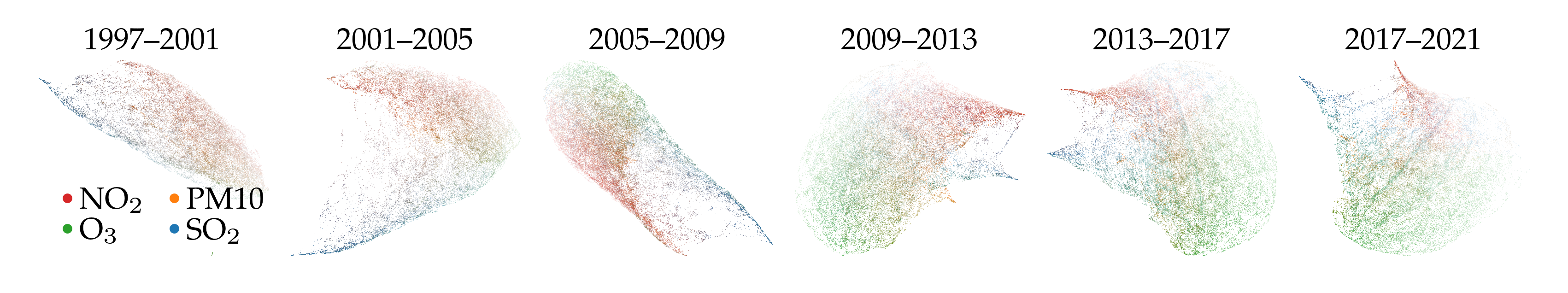
Another alternative is creating multiple UMAP models for different intervals of a signal. For example, below are six embeddings for different periods of time.

A difference between this approach and the year lens is that the interval embeddings do not describe how which points are similar between the intervals. Lining up similar points across the embeddings is possible with the AlignedUMAP class, assuming there is a data point overlap between consecutive intervals. However, that UMAP variant is not GPU accelerated. Here, we use a consistent color for the highest feature to detect similarities between intervals instead.

Another difference is the overall compute cost. Computing multiple smaller UMAP models was twice as fast as computing the full model and applying a lens over the year. However, if the full UMAP model is available, then applying the lens is considerably quicker.

bins = np.arange(df.obs["year"].min(), df.obs["year"].max() + 4, 4)

sized_fig(1, 1 / 6, dpi=600)
plt.subplots_adjust(0, 0, 1, 0.85, 0, 0)
timer = 0
for i, (lower, upper) in enumerate(zip(bins[:-1], bins[1:])):
    sub_df = df[df.obs["year"].between(lower, upper)].copy()
    start_time = time.perf_counter()
    compute_projection(
        sub_df,
        "binned",
        n_neighbors=25,
        repulsion_strengths=[0.001, 0.01, 0.1, 1, 1, 1, 0.2],
        verbose=False,
    )
    end_time = time.perf_counter()
    timer += end_time - start_time
    plt.subplot(1, 6, i + 1)
    plot_category(
        sub_df,
        color="feature",
        layout="binned",
        baseline=-0.3,
        min_alpha=40,
        legend_cols=int(i == 0) * 2,
    )
    plt.title(f"{lower}--{upper}", fontsize=8, y=0.9)
plt.savefig("figures/air_year_intervals.pdf", pad_inches=0)
plt.show()
print(f"Time to compute binned projections: {timer:.2f}s")

Time to compute binned projections: 8.00s

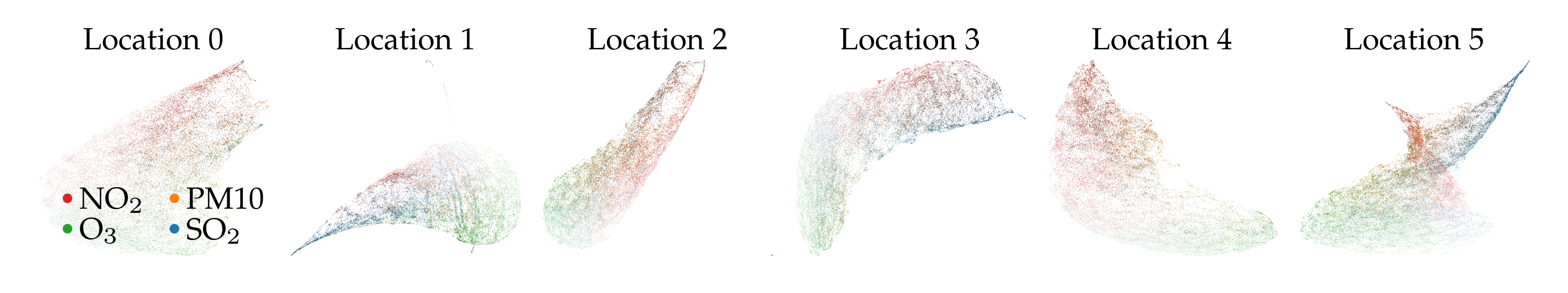
Another small multiple example showing 6 k-means GPS coordinate clusters. The main difference between these clusters appears to relate to time. Clusters with only new locations do not have a high SO2 and NO2 tail.

from sklearn.cluster import KMeans

gps_clusters = KMeans(n_clusters=6).fit_predict(df.obs[["latitude", "longitude"]])

sized_fig(1, 1 / 6, dpi=600)
plt.subplots_adjust(0, 0, 1, 0.85, 0, 0)
timer = 0
for i in range(6):
    sub_df = df[gps_clusters == i].copy()
    start_time = time.perf_counter()
    compute_projection(
        sub_df,
        "binned",
        n_neighbors=25,
        repulsion_strengths=[0.001, 0.01, 0.1, 1, 1, 1, 0.2],
        verbose=False,
    )
    end_time = time.perf_counter()
    timer += end_time - start_time
    plt.subplot(1, 6, i + 1)
    plot_category(
        sub_df,
        color="feature",
        layout="binned",
        baseline=-0.3,
        min_alpha=40,
        legend_cols=int(i == 0) * 2,
    )
    plt.title(f"Location {i}", fontsize=8, y=0.9)
plt.savefig("figures/air_gps_intervals.pdf", pad_inches=0)
plt.show()
print(f"Time to compute binned projections: {timer:.2f}s")

Time to compute binned projections: 6.14s

Weighted distances

Another alternative is emphasizing or including particular features in the input data.

For example, emphasizing the SO2 feature before computing UMAP provides similar embedding as the SO2 local mask. However, tuning the feature strength requires re-computing the full UMAP model, taking +/- 10 seconds, while the applying the year lens takes less than 2 seconds.

df.layers["extra_sulfer"] = df.X.copy()
df[:, "SO2"].layers["extra_sulfer"] *= 2

p_sulfer_dist = compute_projection(
    df,
    "extra_sulfer",
    n_neighbors=50,
    input=df.layers["extra_sulfer"],
)

Build UMAP model: 10.79s
Compute layout: 2.61s

sized_fig(1, 0.618 / 3 + 0.618 / 6)
plot_overview(df, "extra_sulfer")
plt.show()

The same does not hold for emphasizing the Ozon feature, which produces a markedly different embedding when emphasized in the input.

df.layers["extra_ozon"] = df.X.copy()
df[:, "O3"].layers["extra_ozon"] *= 2

p_ozon_dist = compute_projection(
    df, "extra_ozon", n_neighbors=50, input=df.layers["extra_ozon"]
)

Build UMAP model: 10.85s
Compute layout: 2.53s

sized_fig(1, 0.618 / 3 + 0.618 / 6)
plot_overview(df, "extra_ozon")
plt.show()

Similarly, adding the year dimension as feature in the distance computation does not produce an embedding similar to the year lens. Instead, observations in the same year move closer together, overruling the structure that was there without the year feature in the distance.

X_with_year = np.column_stack(
    (df.X, 1.5 * RobustScaler().fit_transform(df.obs.year.values[:, None]))
)

p_year_dist = compute_projection(df, "extra_year", n_neighbors=50, input=X_with_year)

Build UMAP model: 10.15s
Compute layout: 2.68s

sized_fig(1, 0.618 / 3 + 0.618 / 6)
plot_overview(df, "extra_year")
plt.show()

Adding the GPS coordinates as feature in the raw data appears to replicate the original structure for +/- 8 overall locations. The resulting embedding does not resemble the GPS local mask.

X_with_gps = np.column_stack(
    (df.X, 0.5 * RobustScaler().fit_transform(df.obs[["latitude", "longitude"]].values))
)

p_gps_dist = compute_projection(df, "extra_gps", n_neighbors=50, input=X_with_gps)

Build UMAP model: 11.61s
Compute layout: 2.76s

sized_fig(1, 0.618 / 3 + 0.618 / 6)
plot_overview(df, "extra_gps")
plt.show()

Save data

# Export the data.
df.write_h5ad("data/generated/new_air_quality.h5ad")