Comparing clustering algorithms

This notebook aims to answer an overarching questions describing FLASC’s behavior:

1. How does FLASC’s branch-detection ability compare to other clustering algorithms in terms of accuracy and stability?

We compare the algorithms (using tuned parameter settings) on a synthetic dataset in which clusters have branches and for which we have ground-truth branch-membership information. We measure the adjusted rand index (ARI) between the ground-truth and their detected subgroups to describe how well the algorithms segmented the points into the true branch-based subgroups. We measure how much the detected sub-group centroids move between repeated runs to describe the algorithm’s stability (across runs).

%load_ext autoreload
%autoreload 2

import os

# Avoid multi-threading
os.environ["OMP_NUM_THREADS"] = "1"
os.environ["MKL_NUM_THREADS"] = "1"

import numpy as np
import pandas as pd
import matplotlib.pyplot as plt
import seaborn as sns
from lib.plotting import *
%matplotlib inline
configure_matplotlib()

from tqdm import tqdm
from itertools import product
from collections import defaultdict

from scipy import linalg
from sklearn.utils import shuffle
from sklearn.metrics.cluster import adjusted_rand_score

from lib.cdc import CDC
from hdbscan import HDBSCAN
from sklearn.cluster import KMeans, AgglomerativeClustering, SpectralClustering
from flasc import FLASC
from flasc.prediction import (
    branch_centrality_vectors,
    update_labels_with_branch_centrality,
)

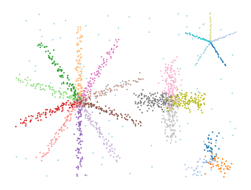
Dataset generation

• Generate multiple star-like clusters spread in 2D space.

• Exponentially spaced points along the branches make density maxima within them unlikely.

• Gaussian noise is added in a varying number of dimensions >= 2.

• Number of points in each branch is varied.

• Uniformly spread noise points are added and given a single target label (num noise points = num points // 20).

def make_star(
    num_dimensions=2,
    num_branches=3,
    points_per_branch=100,
    branch_length=2,
    noise_scale=0.02,
):
    """Creates a n-star in d dimensions."""

    def rotation(axis=[0, 0, 1], theta=0):
        return linalg.expm(np.cross(np.eye(3), axis / linalg.norm(axis) * theta))

    def rotate(X, axis=[0, 0, 1], theta=0):
        M = rotation(axis=axis, theta=theta)
        data = np.hstack((X, np.zeros((X.shape[0], 1), dtype=X.dtype)))
        return (M @ data.T).T[:, :2]

    max_exp = np.log(branch_length)
    branch = np.zeros((points_per_branch, 2))
    branch[:, 0] = np.exp(np.linspace(0, max_exp, points_per_branch)) - 1
    branches = np.concatenate(
        [
            rotate(branch, theta=theta)
            for theta in np.linspace(0, 2 * np.pi, num_branches, endpoint=False)
            + np.pi / 2
        ]
    )
    X = np.column_stack((branches, np.zeros((branches.shape[0], num_dimensions - 2))))
    X += np.random.normal(
        scale=np.sqrt(1 / num_dimensions) * noise_scale,
        size=X.shape,
    )
    y = np.repeat(np.arange(num_branches), points_per_branch)
    return X, y


def make_stars_dataset(size_factor=1, num_dimensions=2):
    num_branches = [3, 10, 4, 5]
    branch_lengths = [1.8, 3.5, 2.3, 2]
    points_per_branch = [40, 100, 150, 20]
    noise_scales = [0.2, 0.1, 0.2, 0.02]
    origins = np.array(
        [
            [7, 1],
            [2, 3],
            [5.5, 3],
            [7, 5],
        ]
    )

    # Make individual starts
    Xs, ys = zip(
        *[
            make_star(
                num_dimensions=num_dimensions,
                num_branches=nb,
                branch_length=l,
                points_per_branch=int(np * size_factor),
                noise_scale=s,
            )
            for l, np, nb, s in zip(
                branch_lengths, points_per_branch, num_branches, noise_scales
            )
        ]
    )

    # Concatenate to one dataset
    X = np.concatenate(
        [
            x + np.concatenate((o, np.zeros(num_dimensions - 2)))
            for x, o in zip(Xs, origins)
        ]
    )
    y = np.concatenate(
        [y + nb for y, nb in zip(ys, [0] + np.cumsum(num_branches).tolist())]
    )

    # Add uniform noise points
    num_noise_points = X.shape[0] // 20
    noise_points = np.random.uniform(
        low=X.min(axis=0), high=X.max(axis=0), size=(num_noise_points, num_dimensions)
    )
    noise_labels = np.repeat(-1, num_noise_points)
    X = np.concatenate((X, noise_points))
    y = np.concatenate((y, noise_labels))

    # Shuffle the data
    return shuffle(X, y), num_noise_points

(X, y), n = make_stars_dataset()
plot_kwargs = dict(s=5, cmap="tab20", vmin=0, vmax=19, edgecolors="k", linewidths=0)
plt.scatter(*X.T, c=y % 20, **plot_kwargs)
plt.axis("off")
plt.show()

Parameter Sweep

A parameter grid-search is used to find the optimal parameters for each algorithm. This ensures we are comparing the algorithms on their best performance. Searching all parameter combinations for all algorithms creates a too large search space. Instead we chose to keep some values at their defaults. We tried to mimic realistic use of the algorithms when selecting which parameters to keep at their default!

algorithms = dict(
    hdbscan=HDBSCAN,
    slink=AgglomerativeClustering,
    cdc=CDC,
    kmeans=KMeans,
    spectral=SpectralClustering,
    flasc=FLASC,
)
static_params = defaultdict(
    dict, slink=dict(linkage="single"), spectral=dict(assign_labels="cluster_qr")
)

# Configure the parameter sweep
n_clusters = np.ceil(np.linspace(4, 27, 6)).astype(np.int32)
n_neighbors = np.round(np.linspace(2, 20, 6)).astype(np.int32)
min_cluster_sizes = np.unique(
    np.round(np.exp(np.linspace(np.log(20), np.log(100), 10)))
).astype(np.int32)
min_branch_sizes = np.unique(
    np.round(np.exp(np.linspace(np.log(3), np.log(50), 10)))
).astype(np.int32)
selection_methods = ["eom", "leaf"]

dynamic_params = dict(
    cdc=dict(k=n_neighbors, ratio=np.linspace(0.5, 0.95, 5).round(2)),
    kmeans=dict(n_clusters=n_clusters),
    slink=dict(n_clusters=n_clusters),
    spectral=dict(n_clusters=n_clusters),
    hdbscan=dict(
        min_samples=n_neighbors,
        min_cluster_size=min_cluster_sizes,
        cluster_selection_method=selection_methods,
    ),
    flasc=dict(
        min_samples=n_neighbors,
        min_cluster_size=min_cluster_sizes,
        min_branch_size=min_branch_sizes,
        cluster_selection_method=selection_methods,
        branch_detection_method=["full", "core"],
    ),
)

all_params = {name for params in dynamic_params.values() for name in params.keys()}

# Create output structure
results = {
    "repeat": [],
    "d": [],
    "alg": [],
    "ari": [],
    "labels": [],
    **{name: [] for name in all_params},
}

for r in tqdm(range(5)):
    for d in [2, 8, 16]:
        # Generate dataset
        (X, y), _ = make_stars_dataset(size_factor=1, num_dimensions=d)
        np.save(f"data/generated/star_parameter_sweep_X_{r}_{d}", X)
        np.save(f"data/generated/star_parameter_sweep_y_{r}_{d}", y)

        # Run the parameter sweep
        for alg_name, alg_class in algorithms.items():
            if alg_name == "cdc" and d > 2:
                continue

            kwargs = static_params[alg_name]
            dynamic_ranges = dynamic_params[alg_name]
            for values in product(*dynamic_ranges.values()):
                params = {
                    param: value for param, value in zip(dynamic_ranges.keys(), values)
                }
                if alg_name == "flasc":
                    params["branch_selection_method"] = params[
                        "cluster_selection_method"
                    ]

                cc = alg_class(**kwargs, **params)
                labels = cc.fit_predict(X)
                if alg_name == "flasc":
                    labels = update_labels_with_branch_centrality(
                        cc, branch_centrality_vectors(cc)
                    )[0]

                results["repeat"].append(r)
                results["d"].append(d)
                results["alg"].append(alg_name)
                results["ari"].append(adjusted_rand_score(y, labels))
                results["labels"].append(labels)
                for name in all_params:
                    results[name].append(params.get(name, np.nan))

# Store the results!
result_df = pd.DataFrame.from_dict(results)
result_df.to_parquet("data/generated/star_parameter_sweep_results.parquet")

100%|██████████| 5/5 [37:41<00:00, 452.30s/it]

Results

Now we visualize the algorithms’ clusters using the best parameter values we found.

result_df = pd.read_parquet("data/generated/star_parameter_sweep_results.parquet")
avg_df = result_df.query("repeat == 0")[["alg", "d", *all_params]].copy()
avg_df["ari"] = np.mean(
    np.stack([result_df.query("repeat == @i").ari.values for i in range(5)]),
    axis=0,
)
best_cases = avg_df.loc[
    avg_df.groupby(["alg", "d"]).apply(lambda x: x.index[np.argmax(x.ari)]).values
]

C:\Users\jelme\AppData\Local\Temp\ipykernel_20084\719546194.py:8: DeprecationWarning: DataFrameGroupBy.apply operated on the grouping columns. This behavior is deprecated, and in a future version of pandas the grouping columns will be excluded from the operation. Either pass `include_groups=False` to exclude the groupings or explicitly select the grouping columns after groupby to silence this warning.
  avg_df.groupby(["alg", "d"]).apply(lambda x: x.index[np.argmax(x.ari)]).values

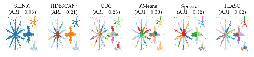
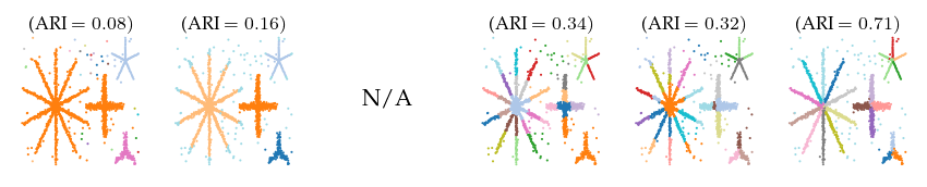
Detected clusters

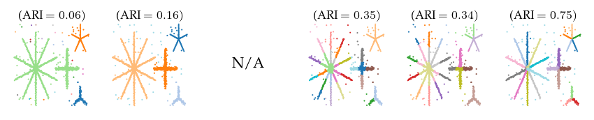
First, lets look at the detected clusters (and branches). Only FLASC is able to reliably find the branches as a distinct subgroup, resulting in ARI scores greater than 0.5. The other algorithms all perform worse.

algs = ["slink", "hdbscan", "cdc", "kmeans", "spectral", "flasc"]
names = ["SLINK", "HDBSCAN*", "CDC", "KMeans", "Spectral", "FLASC"]

for d in result_df.d.unique():
    cnt = 1
    fig = sized_fig(1, 0.2)
    X = np.load(f"data/generated/star_parameter_sweep_X_0_{d}.npy")
    for alg, alg_name in zip(algs, names):
        plt.subplot(1, 6, cnt)
        plt.xticks([])
        plt.yticks([])
        plt.gca().spines["top"].set_visible(False)
        plt.gca().spines["right"].set_visible(False)
        plt.gca().spines["bottom"].set_visible(False)
        plt.gca().spines["left"].set_visible(False)
        cnt += 1
        row = best_cases.query("d == @d and alg == @alg")
        if row.shape[0] == 0:
            plt.text(0.5, 0.5, "N/A", fontsize=10, ha="center", va="center")
            continue
        if d == 2:
            plt.title(f"{alg_name}\n(ARI$={row.ari.iloc[0]:.2f})$", fontsize=8, y=0.92)
        else:
            plt.title(f"(ARI $={row.ari.iloc[0]:.2f})$", fontsize=8, y=0.92)

        plt.scatter(
            *X[:, :2].T,
            s=1,
            c=result_df.loc[row.index, 'labels'].iloc[0] % 20,
            cmap="tab20",
            vmin=0,
            vmax=19,
            edgecolors="none",
            linewidths=0,
        )

    plt.subplots_adjust(bottom=0, left=0, right=1, top=0.78)
    plt.savefig(f'images/star_clusters_{d}.pdf', pad_inches=0)
    plt.show()

ARI over parameters

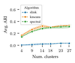
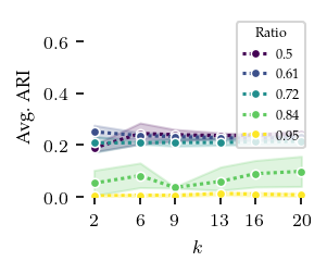
Now, lets explore how sensitive the algorithms are to their parameters. The other algorithms have ARI scores lower than 0.4 regardless of their parameters, and there does not appear to be a trend indicating lower or higher values than tested would improve their performance.

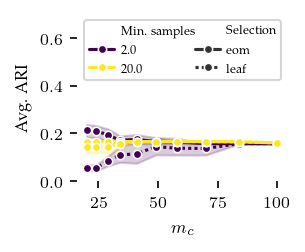
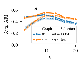
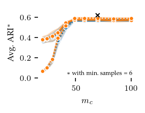
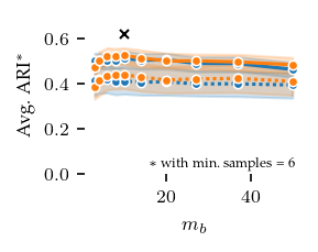
FLASC is most sensitive to the min_samples parameter, in particular with the core approximation graph, which controls the level of connectivity used to extract branches. The more edges are included, the shorter branches are in the graph, leading to a lower branch detection sensitivity. The min_cluster_size and min_branch_size parameters show a different trend. Once their value is large enough to exclude noise, performance remains stable for a longer value range. The optimal combination of these parameters is only visible when looking at the maximum ARI instead of the average ARI shown in the plots.

sized_fig(0.33, aspect=0.8)
sns.lineplot(
    result_df[~np.isnan(result_df.n_clusters)].query("d==2"),
    x="n_clusters",
    y="ari",
    hue="alg",
    dashes=(1, 1),
    marker="o",
    markersize=4,
)
plt.legend(title="Algorithm", handletextpad=0.5, loc="upper left")
plt.xticks(n_clusters)
plt.yticks([0, 0.2, 0.4, 0.6])
plt.ylim(0, 0.7)
plt.xlabel("Num. clusters")
plt.ylabel("Avg. ARI")
plt.show()

sized_fig(0.33, aspect=0.8)
sns.lineplot(
    result_df.query('d == 2 and alg == "cdc"'),
    x="k",
    y="ari",
    hue="ratio",
    dashes=(1, 1),
    markersize=4,
    marker="o",
    palette="viridis",
)
plt.legend(title="Ratio", handletextpad=0.5, loc="upper right")
plt.xticks(n_neighbors)
plt.xlabel("$k$")
plt.ylabel("Avg. ARI")
plt.yticks([0, 0.2, 0.4, 0.6])
plt.ylim(0, 0.7)
plt.show()

samples = [2, 20]
sized_fig(0.33, aspect=0.8)
sns.lineplot(
    result_df.query("d == 2 and alg == 'hdbscan' and min_samples in @samples").rename(
        columns=dict(min_samples="Min. samples", cluster_selection_method="Selection")
    ),
    style="Selection",
    dashes=["", (1, 1)],
    marker="o",
    markersize=4,
    x="min_cluster_size",
    y="ari",
    hue="Min. samples",
    palette="viridis",
)
legend = plt.legend(ncols=2, columnspacing=0, handlelength=2, handletextpad=0.5)
plt.xlabel("$m_c$")
plt.ylabel("Avg. ARI")
plt.yticks([0, 0.2, 0.4, 0.6])
plt.ylim(0, 0.7)
plt.show()

sized_fig(0.33, aspect=0.8)
sns.lineplot(
    result_df.query("d == 2 and alg=='flasc'")
    .rename(
        columns=dict(
            cluster_selection_method="Selection",
            branch_detection_method="Graph",
        )
    )
    .replace(dict(Selection=dict(eom="EOM"))),
    style="Selection",
    dashes=["", (1, 1)],
    marker="o",
    markersize=4,
    x="min_samples",
    y="ari",
    # errorbar=('sd', 1),
    hue="Graph",
    palette="tab10",
)
best = best_cases.query("d == 2 and alg == 'flasc'")
plt.plot(best.min_samples, best.ari, "x", color="black", markersize=4)
legend = plt.legend(
    columnspacing=0,
    handlelength=2,
    handletextpad=0.5,
    loc="lower right",
    ncols=2,
)
adjust_legend_subtitles(legend)
# plt.title("FLASC")
plt.xlabel("$k$")
plt.ylabel("Avg. ARI")
plt.yticks([0, 0.2, 0.4, 0.6])
plt.ylim(0, 0.7)
plt.subplots_adjust(top=1, right=0.97, bottom=0.34, left=0.24)
plt.savefig("images/star_flasc_min_samples.pdf", pad_inches=0)
plt.show()

sized_fig(0.33, aspect=0.8)
sns.lineplot(
    result_df.query("d == 2 and alg=='flasc' and min_samples == 6").rename(
        columns=dict(
            cluster_selection_method="Selection",
            branch_detection_method="Graph",
        )
    ),
    style="Selection",
    dashes=["", (1, 1)],
    marker="o",
    markersize=4,
    # errorbar=("sd", 1),
    x="min_cluster_size",
    y="ari",
    hue="Graph",
    palette="tab10",
    legend=False,
)
plt.plot(best.min_cluster_size, best.ari, "x", color="black", markersize=4)
adjust_legend_subtitles(legend)
plt.xlabel("$m_c$")
plt.ylabel("Avg. ARI$^*$")
plt.text(
    0.95,
    0.35,
    "$*$ with min. samples = 6",
    fontsize=6,
    ha="right",
    va="bottom",
    transform=plt.gcf().transFigure,
)
plt.yticks([0, 0.2, 0.4, 0.6])
plt.ylim(0, 0.7)
plt.subplots_adjust(top=1, right=0.97, bottom=0.34, left=0.24)
plt.savefig('images/star_flasc_min_cluster_size.pdf', pad_inches=0)
plt.show()

sized_fig(0.33, aspect=0.8)
sns.lineplot(
    result_df.query("d==2 and alg=='flasc' and min_samples == 6").rename(
        columns=dict(
            cluster_selection_method="Selection",
            branch_detection_method="Graph",
        )
    ),
    style="Selection",
    dashes=["", (1, 1)],
    marker="o",
    markersize=4,
    # errorbar=("sd", 1),
    x="min_branch_size",
    y="ari",
    hue="Graph",
    palette="tab10",
    legend=False,
)
plt.plot(best.min_branch_size, best.ari, "x", color="black", markersize=4)
adjust_legend_subtitles(legend)
plt.xlabel("$m_b$")
plt.ylabel("Avg. ARI$^*$")
plt.text(
    0.95,
    0.35,
    "$*$ with min. samples = 6",
    fontsize=6,
    ha="right",
    va="bottom",
    transform=plt.gcf().transFigure,
)
plt.yticks([0, 0.2, 0.4, 0.6])
plt.ylim(0, 0.7)
plt.subplots_adjust(top=1, right=0.97, bottom=0.34, left=0.24)
plt.savefig('images/star_flasc_min_branch_size.pdf', pad_inches=0)
plt.show()

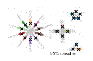
Stability: Centroid spread

To show FLASC provides a stable result (in a practical sense), we visualize the cluster centers it found across the five (random) generated datasets. This demonstrates FLASC’s output is similar across input samples drawn from the same underlying distribution. Other algorithms, like k-means, do not have this property!

from sklearn.metrics import pairwise_distances

centroids = {}
true_centroids = []
flasc_df = result_df.query("alg == 'flasc'").copy()
for r in tqdm(range(flasc_df.repeat.max() + 1)):
    for d in np.unique(flasc_df.d):
        X = np.load(f"data/generated/star_parameter_sweep_X_{r}_{d}.npy")
        y = np.load(f"data/generated/star_parameter_sweep_y_{r}_{d}.npy")

        true_centroid = [np.average(X[y == l], axis=0) for l in np.unique(y) if l != -1]
        true_centroids.append(dict(repeat=r, d=d, centroids=true_centroid))

        for index in flasc_df.query("d==@d and repeat==@r").index:
            labels = flasc_df.loc[index, "labels"]
            found_centroids = np.asarray(
                [
                    np.average(X[labels == l], axis=0)
                    for l in np.unique(labels)
                    if l != -1
                ]
            )
            closest_centroid = np.argmin(
                pairwise_distances(found_centroids, true_centroid), axis=0
            )
            points = found_centroids[closest_centroid]
            centralized_centroids = points - true_centroid
            spread = pairwise_distances(
                np.repeat(0.0, d)[None, :], centralized_centroids
            )[0, :]

            centroids[index] = dict(
                centroids=found_centroids,
                closest_centroid=found_centroids[closest_centroid],
                centralized_centroids=centralized_centroids,
                spread=spread,
            )

true_centroids = pd.DataFrame.from_records(true_centroids)
found_centroids = pd.DataFrame.from_records([*centroids.values()])
found_centroids.index = centroids.keys()
flasc_df = flasc_df.join(found_centroids)

100%|██████████| 5/5 [00:20<00:00,  4.14s/it]

spread = (
    flasc_df.groupby(
        by=[
            "d",
            "min_samples",
            "min_cluster_size",
            "min_branch_size",
            "branch_detection_method",
            "cluster_selection_method",
        ]
    )
    .agg(
        spread=pd.NamedAgg(column="spread", aggfunc=np.vstack),
        centroids=pd.NamedAgg(column="centroids", aggfunc=np.vstack),
        closest_centroid=pd.NamedAgg(column="closest_centroid", aggfunc=np.vstack),
    )
    .reset_index()
)
spread["percentile_95"] = spread.spread.apply(lambda x: np.percentile(x, 95))

Results

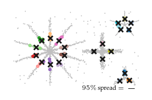
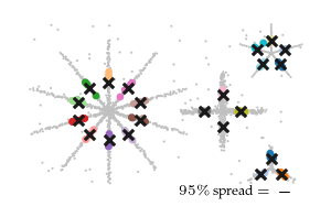
Detected spread

The figure below shows the closest detected centroid (coloured dots) to each ground-truth centroid (black cross) for all five input datasets. Generally, the detected centroids spread around the ground truth centroids, staying within the branch they belong to.

for d in result_df.d.unique():
    fig = sized_fig(0.33)
    X = np.load(f"data/generated/star_parameter_sweep_X_0_{d}.npy")
    truths = np.asarray(
        true_centroids.query("d == @d and repeat == 0").centroids.iloc[0]
    )

    plt.xticks([])
    plt.yticks([])
    plt.gca().spines["top"].set_visible(False)
    plt.gca().spines["right"].set_visible(False)
    plt.gca().spines["bottom"].set_visible(False)
    plt.gca().spines["left"].set_visible(False)

    best_settings = best_cases.query('alg=="flasc" and d == 2').iloc[0]
    row = spread.query(
        "d == @d and "
        "min_samples == @best_settings.min_samples and "
        "cluster_selection_method == @best_settings.cluster_selection_method and "
        "branch_detection_method == @best_settings.branch_detection_method and "
        "min_cluster_size == @best_settings.min_cluster_size and "
        "min_branch_size == @best_settings.min_branch_size"
    )

    centroid = row.closest_centroid.iloc[0][:, :2]
    plt.scatter(*X[:, :2].T, s=1, color="silver", edgecolors="none", linewidths=0)
    plt.scatter(
        *centroid.T,
        s=5,
        c=[i % 20 for _ in range(5) for i in range(truths.shape[0])],
        marker="o",
        cmap="tab20",
        vmin=0,
        vmax=19,
    )
    plt.scatter(*truths[:, :2].T, s=20, color="k", marker="x")
    plt.text(
        0.85,
        0.01,
        f"$95\%$ spread $ = $",
        ha="right",
        va="bottom",
        fontsize=6,
        transform=plt.gcf().transFigure,
    )
    mid = 7.25
    plt.plot(
        [mid, mid + row.percentile_95.iloc[0]],
        [0.2, 0.2],
        color="black",
        linewidth=0.5,
    )


    plt.subplots_adjust(left=0, right=1, top=1, bottom=0)
    plt.savefig(f'images/star_spread_{d}.pdf', pad_inches=0)
    plt.show()

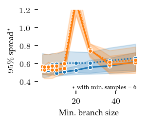
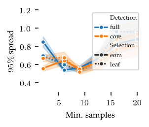
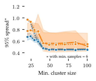
Spread over parameters

The distances between these closest detected centroids and their corresponding ground truth centroid can also be used to explore parameter sensitive. Here, we show the 95th percentile distance over true centroids across all five repeats. Lower values are better. The parameters show approximately the same pattern as with the ARI. Note that this measure is too optimistic when FLASC finds more than the true number of subgroups.

sized_fig(0.33, aspect=0.8)
sns.lineplot(
    spread.query("d == 2").rename(
        columns=dict(
            cluster_selection_method="Selection",
            branch_detection_method="Detection",
        )
    ),
    style="Selection",
    dashes=["", (1, 1)],
    marker="o",
    markersize=4,
    x="min_samples",
    y="percentile_95",
    hue="Detection",
    hue_order=["full", "core"],
    palette="tab10",
)
legend = plt.legend(
    columnspacing=0, handlelength=2, handletextpad=0.5, loc="upper right"
)
adjust_legend_subtitles(legend)
plt.xlabel("Min. samples")
plt.ylabel("$95\%$ spread")
ylim = [0.3, 1.2]
plt.ylim(ylim)
plt.show()

sized_fig(0.33, aspect=0.8)
sns.lineplot(
    spread.query("d == 2 and min_samples==6").rename(
        columns=dict(
            cluster_selection_method="Selection",
            branch_detection_method="Detection",
        )
    ),
    style="Selection",
    dashes=["", (1, 1)],
    marker="o",
    markersize=4,
    # errorbar=("pi", 50),
    x="min_cluster_size",
    y="percentile_95",
    hue="Detection",
    hue_order=["full", "core"],
    palette="tab10",
    legend=False,
)
adjust_legend_subtitles(legend)
plt.xlabel("Min. cluster size")
plt.ylabel("$95\%$ spread$^*$")
plt.text(
    0.875,
    0.11,
    "$*$ with min. samples = 6",
    fontsize=6,
    ha="right",
    va="bottom",
    transform=plt.gcf().transFigure,
)
plt.ylim(ylim)
plt.show()

sized_fig(0.33, aspect=0.8)
sns.lineplot(
    spread.query("d==2 and min_samples==6").rename(
        columns=dict(
            cluster_selection_method="Selection",
            branch_detection_method="Detection",
        )
    ),
    style="Selection",
    dashes=["", (1, 1)],
    marker="o",
    markersize=4,
    # errorbar=("pi", 50),
    x="min_branch_size",
    y="percentile_95",
    hue="Detection",
    hue_order=["full", "core"],
    palette="tab10",
    legend=False,
)
adjust_legend_subtitles(legend)
plt.xlabel("Min. branch size")
plt.ylabel("$95\%$ spread$^*$")
plt.text(
    0.875,
    0.11,
    "$*$ with min. samples = 6",
    fontsize=6,
    ha="right",
    va="bottom",
    transform=plt.gcf().transFigure,
)
plt.ylim(ylim)
plt.show()