5. Graph databases
5.1. Introduction
Graphs are used in a wide range of applications, from fraud detection (see the Panama Papers) and anti-terrorism and social marketing to drug interaction research and genome sequencing.
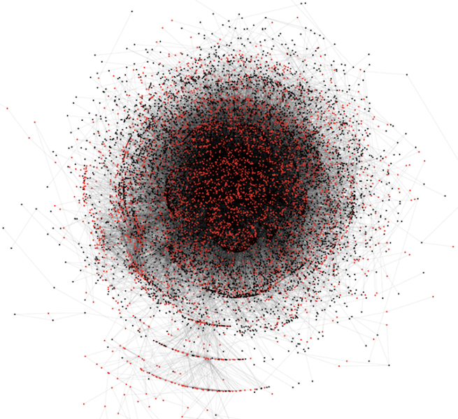
Graphs or networks are data structures where the most important information is the relationship between entities rather than the entities themselves, such as friendship relationships. Whereas in relational databases you typically aggregate operations on sets, in graph databases you’ll more typically hop around relationships between records. Graphs are very expressive, and any type of data can be modelled as one (although that is no guarantee that a particular graph is fit for purpose).
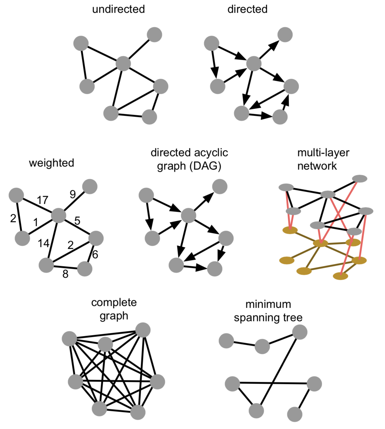
Graphs come in all shapes and forms. Links can be directed or undirected, weighted or unweighted. They can be directed acyclic graphs (where no loops exist), consist of one or more connected components, and actually consist of multiple graphs themselves. The latter (so-called multi-layer networks) can e.g. be a first network representing friendships between people, a second network representing cities and how they are connected through public transportation, and both being linked by which people work in which cities.
5.2. Nomenclature
A graph consists of vertices (aka nodes, aka objects) and edges (aka links, aka relations), where an edge is a connection between two vertices. Both vertices and edges can have properties.
\[G = (V,E)\]
Any graph can be described using different metrics:
-
order of a graph = number of nodes
-
size of a graph = number of edges
-
graph density = how much its nodes are connected. In a dense graph, the number of edges is close to the maximal number of edges (i.e. a fully-connected graph).
-
for undirected graphs, this is: \[\frac{2 |E|}{|V|(|V|-1)}\]
-
for directed graphs, this is: \[\frac{|E|}{|V|(|V|-1)}\]
-
-
the degree of a node = how many edges are connected to the node. This can be separated into in-degree and out-degree, which are - respectively - the number of incoming and outgoing edges.
-
the distance between two nodes = the number of edges in the shortest path between them
-
the diameter of a graph = the maximum distance in a graph
-
a d-regular graph = a graph where the maximum degree is the same as the minimum degree d
-
a path = a sequence of edges that connects a sequence of different vertices
-
a connected graph = a graph in which there exists a direct connection between any two vertices
5.3. Centralities
Another important way of describing nodes is based on their centrality, i.e. how central they are in the network. There exist different versions of this centrality:
-
degree centrality: how many other vertices a given vertex is connected to. This is the same as node degree.
-
betweenness centrality: how many critical paths go through this node? In other words: without these nodes, there would be no way for to neighbours to communicate. \[ C_{B}(i)=\frac{\sum\limits_{j \neq k} g_{jk} (i)}{g_{jk}} \xrightarrow[]{normalize} C'_B = \frac{C_B(i)}{(n-1)(n-2)/2}\] , where the denominator is the number of vertex pairs excluding the vertex itself. \(g_jk(i)\) is number of shortest paths between \(j\) and \(k\), going through i; \(g_jk\) is the total number of shortest paths between \(j\) and \(k\).
-
closeness centrality: how much is the node in the "middle" of things, not too far from the center. This is the inverse total distance to all other nodes. \[C_C(i) = \frac{1}{\sum\limits_{j=1}^N d(i,j)} \xrightarrow[]{normalize} C'_C(i) = \frac{C_C(i)}{N-1}\]
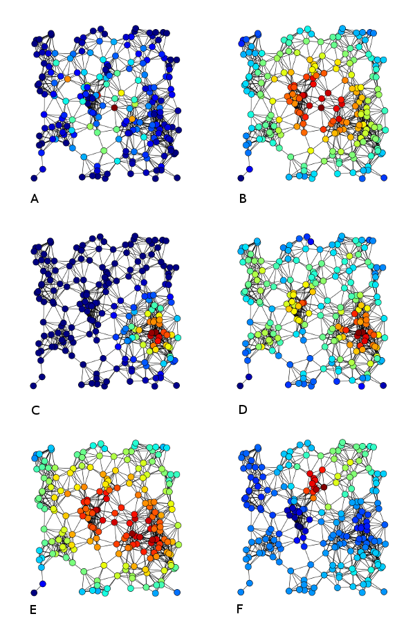
In the image below, nodes in A are coloured based on betweenness centrality, in B based on closeness centrality, and in D on degree centrality.
5.4. Graph mining
Graphs are very generic data structures, but are amenable to very complex analyses. These include the following.
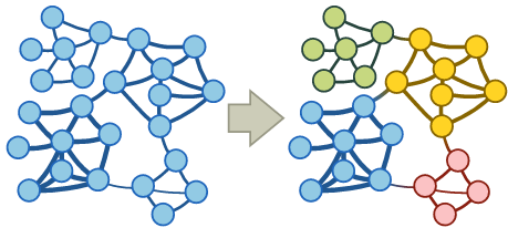
5.4.1. Community detection
A community in a graph is a group of nodes that are densely connected internally. You can imagine that e.g. in social networks we can identify groups of friends this way.
Several approaches exist to finding communities:
-
null models: a community is a set of nodes for which the connectivity deviates the most from the null model
-
block models: identify blocks of nodes with common properties
-
flow models: a community is a set of nodes among which a flow persists for a long time once entered
The infomap algorithm is an example of a flow model (for a demo, see http://www.mapequation.org/apps/MapDemo.html).
5.4.2. Link prediction
When data is acquired from a real-world source, this data might be incomplete and links that should actually be there are not in the dataset. For example, you gather historical data on births, marriages and deaths from church and city records. There is therefore a high chance that you don’t have all data. Another domain where this is important is in protein-protein interactions.
Link prediction can be done in different ways, and can happen in a dynamic or static setting. In the dynamic setting, we try to predict the likelihood of a future association between two nodes; in the static setting, we try to infer missing links. These algorithms are based on a similarity matrix between the network nodes, which can take different forms:
-
graph distance: the length of the shortest path between 2 nodes
-
common neighbours: two strangers who have a common friend may be introduced by that friend
-
Jaccard’s coefficient: the probability that 2 nodes have the same neighbours
-
frequency-weighted common neighbours (Adamic/Adar predictor): counts common features (e.g. links), but weighs rare features more heavily
-
preferential attachment: new link between nodes with high number of links is more likely than between nodes with low number of links
-
exponential damped path counts (Katz measure): the more paths there are between two nodes and the shorter these paths are, the more similar the nodes are
-
hitting time: random walk starts at node A ⇒ expected number of steps required to reach node B
-
rooted pagerank: idem, but periodical reset to prevent that 2 nodes that are actually close are connected through long deviation
5.4.3. Subgraph mapping
Subgraph mining is another type of query that is very important in e.g. bioinformatics. Some example patterns:
-
[A] three-node feedback loop
-
[B] tree chain
-
[C] four-node feedback loop
-
[D] feedforward loop
-
[E] bi-parallel pattern
-
[F] bi-fan
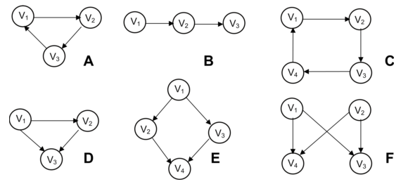
It is for example important when developing a drug for a certain disease by knocking out the effect of a gene that that gene is not in a bi-parallel pattern (V2 in image E above) because activation of node V4 is saved by V3.
5.5. Data modeling
In general, vertices are used to represent things and edges are used to represent connections. Vertex properties can include e.g. metadata such as timestamp, version number etc; edges properties often include the weight of a connection, but can also cover things like the quality of a relationship and other metadata of that relationship.
Below is an example of a graph:
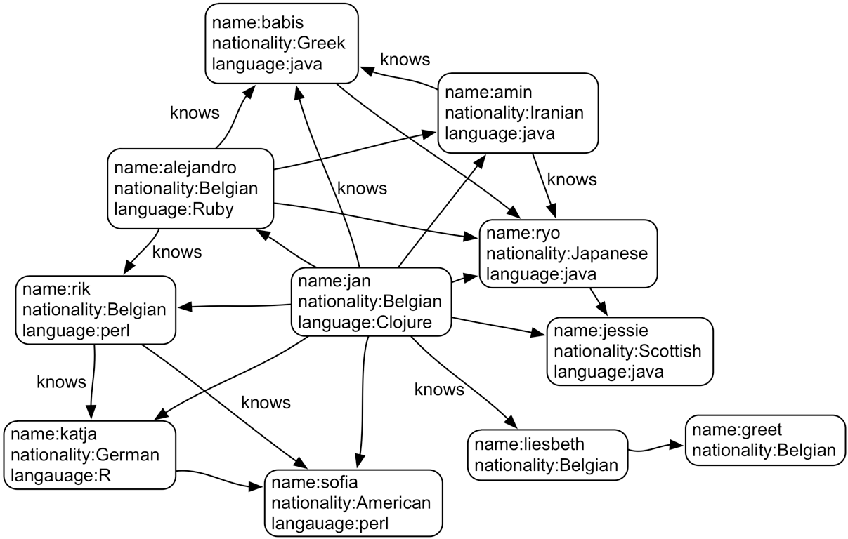
Basically all types of data can be modelled as a graph. Consider our buildings table from above:
| id | name | address | city | type | nr_rooms | primary_or_secondary |
|---|---|---|---|---|---|---|
1 |
building1 |
street1 |
city1 |
hotel |
15 |
|
2 |
building2 |
street2 |
city2 |
school |
primary |
|
3 |
building3 |
street3 |
city3 |
hotel |
52 |
|
4 |
building4 |
street4 |
city4 |
church |
||
5 |
building5 |
street5 |
city5 |
house |
||
… |
… |
… |
… |
… |
… |
… |
This can also be represented as a network, where:
-
every building is a vertex
-
every value for a property is a vertex as well
-
the column becomes the relation
For example, the information for the first building can be represented as such:

There is actually a formal way of describing this called RDF, but we won’t go into that here…