1. Relational Database Management Systems
This is a practical introduction to relational database management systems and SQL. The text is written focussing on how you can get things done, and does not go into the theoretical and technical backgrounds. The online version of this text is available at http://vda-lab.github.io/data-management
Working with data almost invariably involves working with relational databases and SQL (Structured Query Language). They have a decades-old history and are very established. In this section, we go over the why and how of this type of database.
Let’s look at some example life science fields where we collect data to make the rest of the session a bit more concrete.
1.1. Examples of data
1.1.1. Microbiome data
Microbiome data offer a window into the complex world of microbial communities and their interactions with their environment. This can be in the human or animal body, soil, or other ecosystems. By measuring and analyzing this data, we can gain insights into a lot of processes: in humans and animals, it can illuminate aspects of health, disease, and nutrition; in agriculture, it can enhance our understanding of soil health, plant growth, and crop resilience.
Microbiome data typically consist of OTU (operational taxonomic unit) or ASV (amplicon sequence variant) tables, which can be considered large tables where the columns represent the OTUs/ASVs, the rows represent different samples, and the cells indicate the amount of that OTU/ASV found in a particular sample.
| sample | SRS024625.570280 | SRS018102.573993 | SRS017304.575372 | SRS024151.575546 | … |
|---|---|---|---|---|---|
963239 |
12 |
2 |
0 |
15 |
… |
4431292 |
0 |
5 |
1 |
3 |
… |
4480529 |
7 |
0 |
0 |
0 |
… |
4345640 |
0 |
3 |
1 |
8 |
… |
… |
… |
… |
… |
… |
… |
Both samples and OTUs/ASVs themselves can contain metadata. For the samples, these can include the sampling device, the age of the subject, the location of the sample (e.g. skin vs gut vs …), etc. For the OTUs, these are e.g. consensus sequences and taxonomy.
1.1.2. DNA sequencing and genotyping
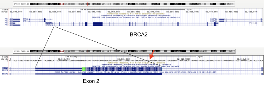
The importance of DNA sequencing and genotyping is steadily increasing within research and health care. In genotyping, one reads the nucleotides at specific positions in the genome to check if the patient has an allele that for example constitutes a higher risk to certain diseases, or that indicates higher or lower sensitivity to certain medication.
For example, mutations in the BRCA1 and BRCA2 genes change a person’s chance of getting breast cancer (see http://arup.utah.edu/database/BRCA/Variants/BRCA2.php for a list of possible mutations in BRCA2 and their pathogenicity). One of the many harmful mutations is a mutation at position 32,316,517 on chromosome 13 (in exon 2 of BRCA2) that changes a C to an A, resulting in a stop codon.
Genotyping results therefore contain information on:
-
the individual
-
the polymorphism (i.e. identifying what nucleotide is changed) position in the genome (i.e. chr13 position 32,316,517)
-
the allele (i.e. C or A)
For each, additional information can be recorded:
-
for the individual: their name, ethnicity
-
for the polymorphism: the unique identifier in a central database (in this case: rs878853592), the chromosome (chr13), the position (32,316,517), the allele that occurs in healthy individuals (i.e. C)
An example genotype table:

This table contains the information for 3 polymorphisms (called rs12345, rs98765 and rs28465) for 2 individuals (individual_A and individual_B). Typically, thousands of polymorphisms are recorded for thousands of individuals.
A particular type of polymorphism is the single nucleotide polymorphism (SNP), which will be why tables below will be called snps.
1.1.3. Epidemiological studies
Epidemiology is described as "the study of the occurrence and distribution of health-related states or events in specified populations, including the study of determinants influencing such states, and the application of this knowledge to control the health problems" (Dictionary of Epidemiology, Porta 2008). It covers a very broad and diverse line of research:
-
experimental vs observational studies
-
within the observational studies:
-
exploratory vs descriptive
-
exposure vs outcome oriented
-
The collected data can also be very diverse, and include questionnaires, forms, medical device outcomes, biological data, etc.
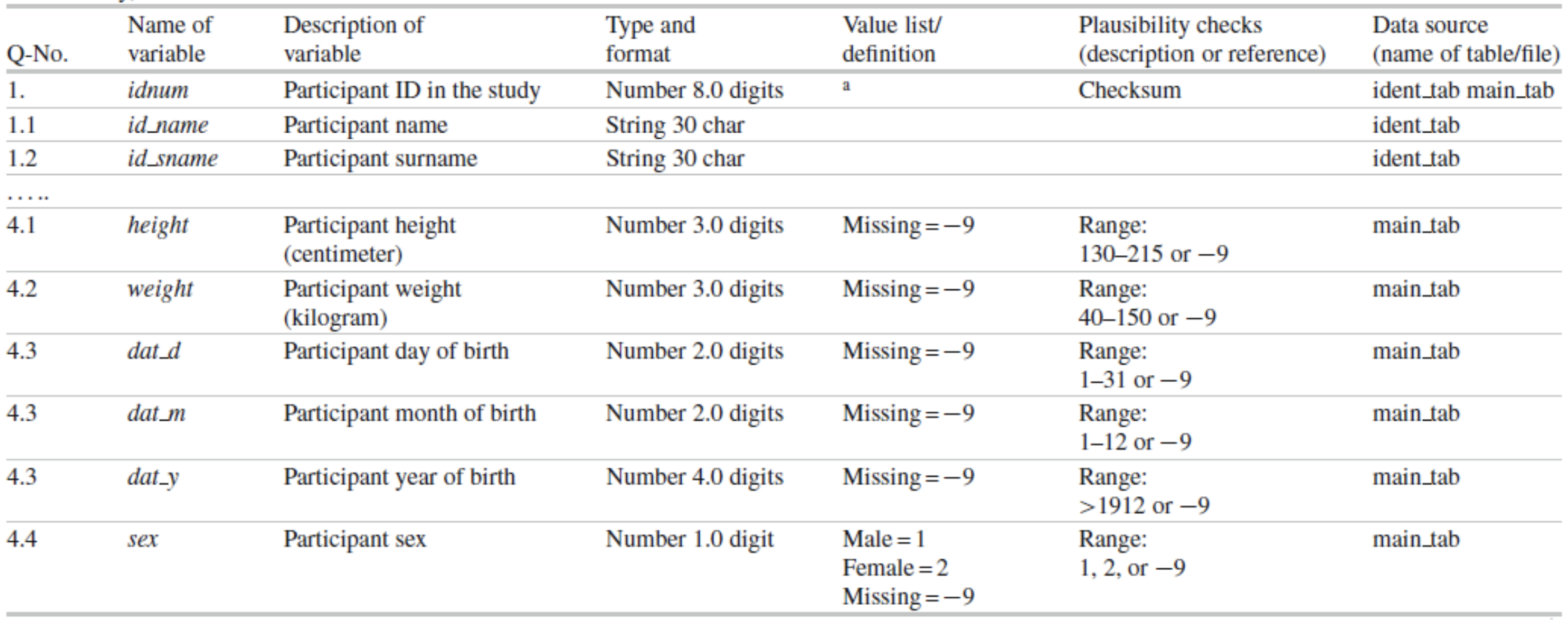
Epidemiological studies are generally done in one of two settings: primary (based on newly collected data) or secondary (using existing databases).
Generally a codebook or data dictionary that describes all data sources (collected, derived, transformed, …). An example of a data dictionary is provided below (taken from Ahrens, W. et al. (2014): Handbook of epidemiology. Table 27.2).
1.2. Relational databases
There is a wide variety of database systems to store data, but the most-used in the relational database management system (RDBMS). These basically consist of tables that contain rows (which represent instance data) and columns (representing properties of that data). Any table can be thought of as an Excel-sheet.
Relational databases are the most wide-spread paradigm used to store data. They use the concept of tables with each row containing an instance of the data, and each column representing different properties of that instance of data. Different implementations exist, include ones by Oracle and MySQL. For many of these (including Oracle and MySQL), you need to run a database server in the background. People (or you) can then connect to that server via a client. In this session, however, we’ll use SQLite3. SQLite is used by Firefox, Chrome, Android, Skype, …
1.2.1. SQLite
The relational database management system (RDBMS) that we will use is SQLite. It is very lightweight and easy to set up.
Using SQLite on the linux command line
To create a new database that you want to give the name 'new_database.sqlite', just call sqlite3 with the new database name. sqlite3 new_database.sqlite The name of that file does not have to end with .sqlite, but it helps you to remember that this is an SQLite database. If you add tables and data in that database and quit, the data will automatically be saved.
There are two types of commands that you can run within SQLite: SQL commands (the same as in any other relational database management system), and SQLite-specific commands. The latter start with a period, and do not have a semi-colon at the end, in contrast to SQL commands (see later).
Some useful commands:
-
.help⇒ Returns a list of the SQL-specific commands -
.tables⇒ Returns a list of tables in the database -
.schema⇒ Returns the schema of all tables -
.header on⇒ Add a header line in any output -
.mode column⇒ Align output data in columns instead of output as comma-separated values -
.quit
Using DB Browser for SQLite
If you like to use a graphical user interface (or don’t work on a linux or OSX computer), you can use the DB Browser for SQLite which you can download here.
Note: In all code snippets that follow below, the sqlite> at the front represents the sqlite prompt, and should not be typed in…
1.3. Database schema and normalisation
We’ll look into two examples to guide us through developing a good database schema. The database schema is basically the description of what the database looks like: what are the names of the tables, what are the columns in those tables, and how are these connected between tables?
1.3.1. A student database
The simplest version
Let’s say we want to store which students follow the G0R72A course ("Data Visualisation in Data Science"). We want to keep track of their first name, last name, student ID, and whether or not they follow the course. This should allow for some easy queries, such as listing all people who take the course, or returning the number of people who do so. In this case, a flat database would suffice; i.e. a single table can hold all information.
| first_name | last_name | student_id | takes_course |
|---|---|---|---|
Martin |
Van Deun |
S0001 |
I0U29A |
Martin |
Van Deun |
S0001 |
I0P18A |
Martin |
Van Deun |
S0001 |
H09B7A |
… |
… |
… |
… |
Martin |
Van Deun |
S0001 |
E02N3A |
Sarah |
Smith |
S0002 |
I0U29A |
… |
… |
… |
… |
A slightly less simple setting
Consider that we want to store which students follow which courses in MSc Statistics. So we’d like to keep:
-
first name, last name, student ID
-
courses a student takes (E02N3A, G0R72A, …)
This should allow for queries e.g. to find out which people follow a particular course, the average number of courses a student takes, etc.
Let’s take the same approach as above, and we simply add a column for each course.
| first_name | last_name | student_id | takes_I0U29A | takes_G0R72A | … | takes_E02N3A |
|---|---|---|---|---|---|---|
Martin |
Van Deun |
S0001 |
Y |
Y |
… |
N |
Sarah |
Smith |
S0002 |
Y |
N |
… |
Y |
Mary |
Kopals |
S0003 |
N |
Y |
… |
Y |
… |
… |
… |
… |
… |
… |
… |
This way of working (called the wide format) does present some issues, though.
-
We will end up with a huge table. Imagine there are 20 courses at KU Leuven and 80 at other universities in Flanders that the student can follow. In addition, suppose there are 50 students. This would mean that we need (3 + 100)*50 = 5,150 cells to store this data.
-
There can be a lot of wasted space, for example courses that nobody takes.
An alternative is to use the long format:
| first_name | last_name | student_id | takes_course |
|---|---|---|---|
Martin |
Van Deun |
S0001 |
I0U29A |
Martin |
Van Deun |
S0001 |
I0P18A |
Martin |
Van Deun |
S0001 |
H09B7A |
… |
… |
… |
… |
Martin |
Van Deun |
S0001 |
E02N3A |
Sarah |
Smith |
S0002 |
I0U29A |
… |
… |
… |
… |
This solves the issue of not having to store the information when a course is not taken, decreasing the number of cells needed from 5,150 to 2,000.
This is still not ideal though, as this design still suffers from a lot of redundancy: the first name, last name and student ID are provided over and over again. Imagine that we’d keep home address (street, street number, zip code, city, country) as well, that would look like this:
| first_name | last_name | student_id | street | number | zip | city | takes_course |
|---|---|---|---|---|---|---|---|
Martin |
Van Deun |
S0001 |
Some Street |
1 |
1234 |
MajorCity |
I0U29A |
Martin |
Van Deun |
S0001 |
Some Street |
1 |
1234 |
MajorCity |
I0P18A |
Martin |
Van Deun |
S0001 |
Some Street |
1 |
1234 |
MajorCity |
H09B7A |
… |
… |
… |
… |
… |
… |
… |
… |
Martin |
Van Deun |
S0001 |
Main Street |
1 |
1234 |
SmallVillage |
E02N3A |
Sarah |
Smith |
S0002 |
Main Street |
1 |
1234 |
SmallVillage |
I0U29A |
… |
… |
… |
… |
… |
… |
… |
… |
What if Martin Van Deun moves from Some Street 1 in MajorCity to Another Street 42 in AnotherCity? Then we would have to edit all the rows in this table that contain this information, which almost guarantees that you will end up with inconsistencies.
1.3.2. A genotype database
Let’s look at another example. Let’s say you want to store individuals and their genotypes. In Excel, you could create a sheet that looks like this with genotypes for 3 polymorphisms in 2 individuals:
| individual | ethnicity | rs12345 | rs12345_amb | chr_12345 | pos_12345 | rs98765 | rs98765_amb | chr_98765 | pos_98765 | rs28465 | rs28465_amb | chr_28465 | pos_28465 |
|---|---|---|---|---|---|---|---|---|---|---|---|---|---|
individual_A |
caucasian |
A/A |
A |
1 |
12345 |
A/G |
R |
1 |
98765 |
G/T |
K |
5 |
28465 |
individual_B |
caucasian |
A/C |
M |
1 |
12345 |
G/G |
G |
1 |
98765 |
G/G |
G |
5 |
28465 |
Let’s actually create this database using the sqlite DB Browser mentioned above.
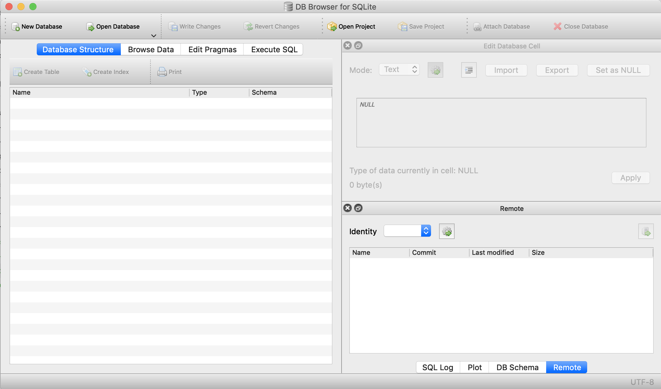
We first select New database and after giving it a name, click Create table. This is where we’ll describe what the columns should be.
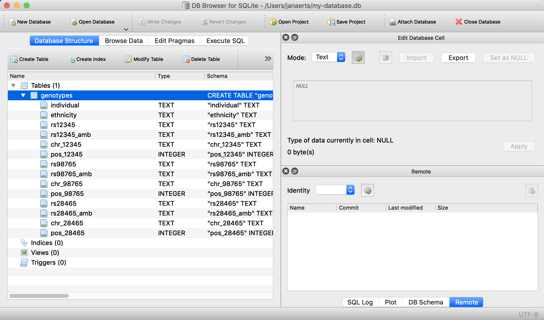
We create a table called genotypes with the following columns:
-
individualof typeTEXT -
ethnicityof typeTEXT -
rs12345of typeTEXT -
rs12345_ambof typeTEXT -
chr_12345of typeTEXT -
pos_12345of typeINTEGER -
rs98765of typeTEXT -
rs98765_ambof typeTEXT -
chr_98765of typeTEXT -
pos_98765of typeINTEGER -
rs28465of typeTEXT -
rs28465_ambof typeTEXT -
chr_28465of typeTEXT -
pos_28465of typeINTEGER
We should now see the following:
This table can also be created using the following SQL command (more on this later):
CREATE TABLE genotypes (individual STRING,
                        ethnicity STRING,
                        rs12345 STRING,
                        rs12345_amb STRING,
                        chr_12345 STRING,
                        pos_12345 INTEGER,
                        rs98765 STRING,
                        rs98765_amb STRING,
                        chr_98765 STRING,
                        pos_98765 INTEGER,
                        rs28465 STRING,
                        rs28465_amb STRING,
                        chr_28465 STRING,
                        pos_28465 INTEGER);
This only sets up the structure. We still need to actually load the data for these two individuals. We will use SQL INSERT statements for this. Click on Execute SQL, paste the code below, and run it.
INSERT INTO genotypes (individual,
                       ethnicity,
                       rs12345,
                       rs12345_amb,
                       chr_12345,
                       pos_12345,
                       rs98765,
                       rs98765_amb,
                       chr_98765,
                       pos_98765,
                       rs28465,
                       rs28465_amb,
                       chr_28465,
                       pos_28465)
           VALUES ('individual_A','caucasian','A/A','A','1',12345, 'A/G','R','1',98765, 'G/T','K','5',28465);
INSERT INTO genotypes (individual,
                       ethnicity,
                       rs12345,
                       rs12345_amb,
                       chr_12345,
                       pos_12345,
                       rs98765,
                       rs98765_amb,
                       chr_98765,
                       pos_98765,
                       rs28465,
                       rs28465_amb,
                       chr_28465,
                       pos_28465)
            VALUES ('individual_B','caucasian','A/C','M','1',12345, 'G/G','G','1',98765, 'G/G','G','5',28465);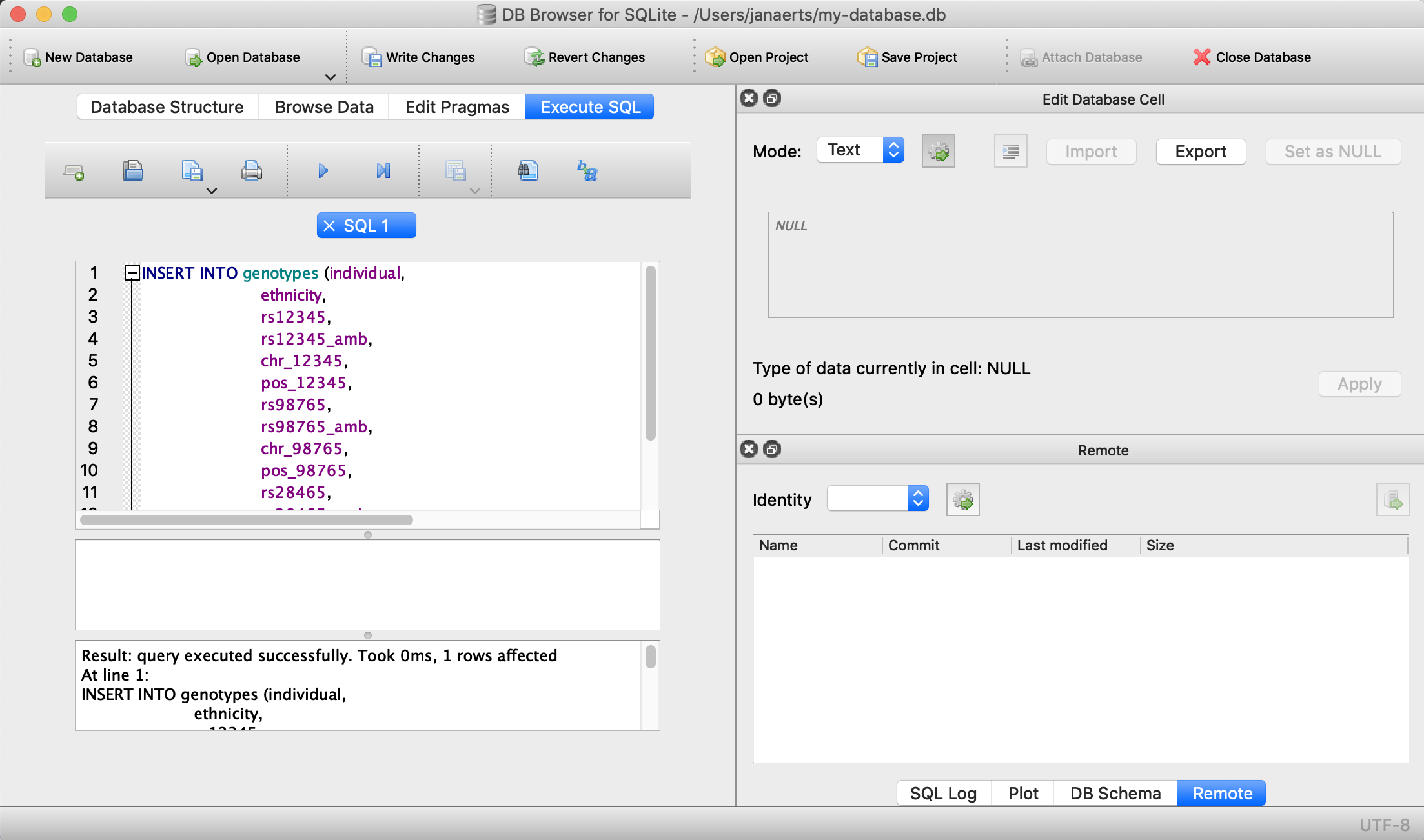
Note that every SQL command is ended with a semi-colon…
We can now check that everything is loaded by clicking on Browse Data (we’ll come back to getting data out later):
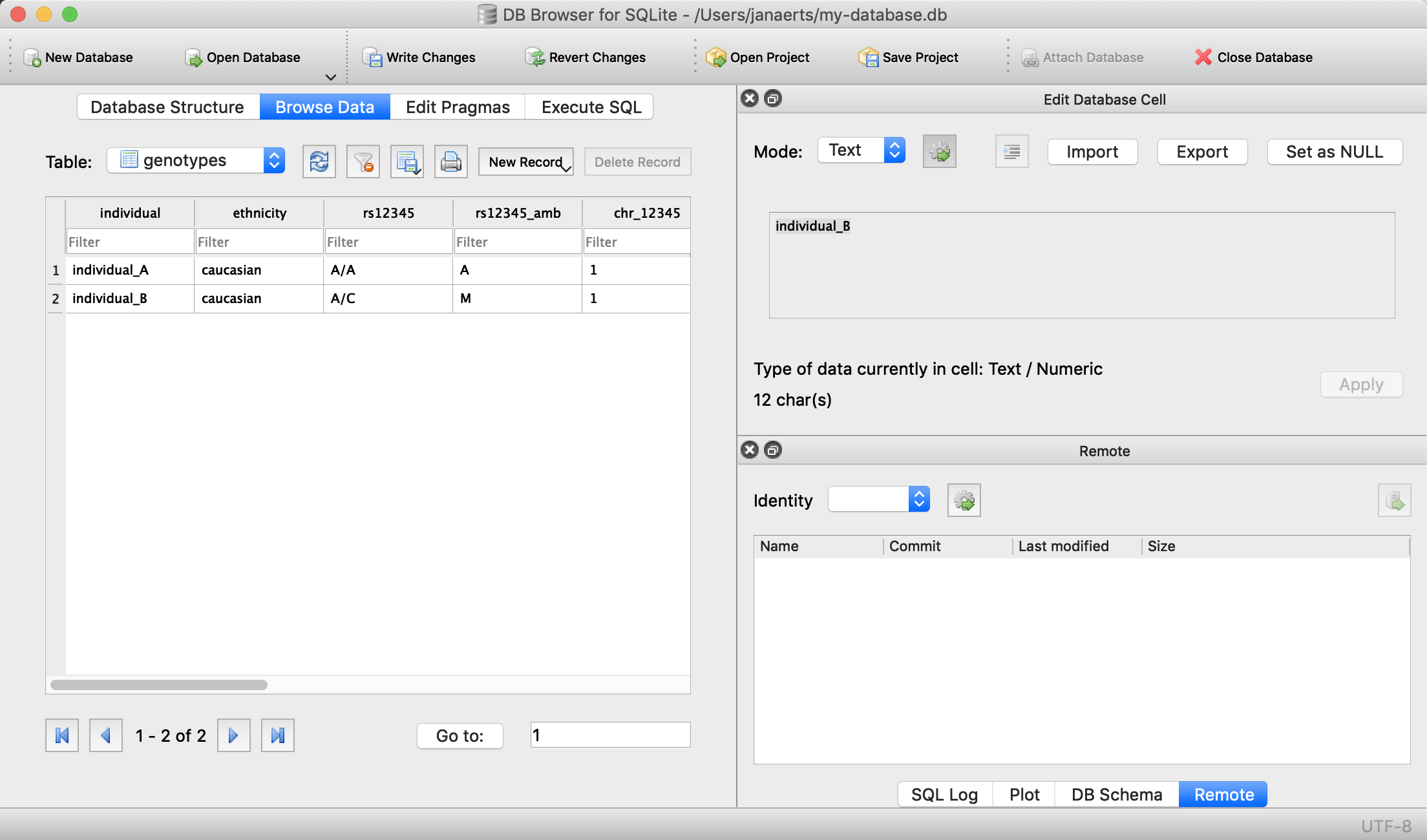
Done! For every new SNP we just add a new column, right? Wrong… In contrast to the student example above where there are - let’s say - 100 courses, a genotyping experiment can return results for millions of positions. Imaging having a table with millions of columns.
1.3.3. Normal forms
There are some good practices in developing relational database schemes which make it easier to work with the data afterwards. Some of these practices are represented in the "normal forms".
Let’s consider the following table listing individuals, SNPs and genotypes. This is genetic data. As you know, everyone has very similar DNA (otherwise we wouldn’t be human), but there are a lot of positions in that genome (about 1/1000) where people differ from each other (otherwise we would all be clones). A "single nucleotide polymorphism" (or "SNP") is such a position in the genome. A "genotype" is the actual nucleotides that someone has in his/her genome at that particular position. And because we have 2 copies of each chromosome, a genotype consists of 2 letters (A, C, G and T).
| individual | ethnicity | rs12345 | chromosome;position | rs12345_diseases | rs98765 | chromosome;position | rs28465 | chromosome;position |
|---|---|---|---|---|---|---|---|---|
individual_A |
caucasian |
A/A |
1;12345 |
COPD;asthma |
A/G |
1;98765 |
G/T |
5;28465 |
individual_B |
caucasian |
A/C |
1;12345 |
COPD;asthma |
G/G |
1;98765 |
G/G |
5;28465 |
First normal form
To get to the first normal form:
-
Make columns atomic: a single cell should contain only a single value
-
Values in a column should be of a single domain: a single column should not have a mix of data
-
All columns should have unique names
-
Columns should be not be hidden lists: often clear because the column name actually holds information
The above table violates several of these points:
-
The
rs12345_diseasescolumns holds non-atomic values:COPD;asthmais a list. -
The column name
chromosome;positionis used multiple times. -
The columns
rs12345,rs98765andrs28465are effectively the same thing: they describe the genotypes for a particular SNP. The same is true for thechromsome;positioncolumns (but that was already clear from the previous point).
The solution to these issues is to go from a wide format to a long format: remove columns by adding rows. For example, the information for the 3 different SNPs is now stored in different rows instead of different columns. The same is true for the non-atomic values: we just duplicate the row to be able to split up the diseases. This will end up with many rows but don’t worry about that.
| individual | ethnicity | snp | genotype | chr | pos | disease |
|---|---|---|---|---|---|---|
individual_A |
caucasian |
rs12345 |
A/A |
1 |
12345 |
COPD |
individual_A |
caucasian |
rs12345 |
A/A |
1 |
12345 |
asthma |
individual_B |
caucasian |
rs12345 |
A/C |
1 |
12345 |
COPD |
individual_B |
caucasian |
rs12345 |
A/C |
1 |
12345 |
asthma |
individual_A |
caucasian |
rs98765 |
A/G |
1 |
98765 |
|
individual_B |
caucasian |
rs98765 |
G/G |
1 |
98765 |
|
individual_A |
caucasian |
rs28465 |
G/T |
5 |
28465 |
|
individual_B |
caucasian |
rs28465 |
G/G |
5 |
28465 |
The new schema:
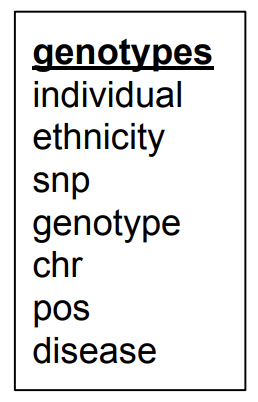
Everything is still contained in a single table, which will change when we go to the second normal form.
Second normal form
-
Schema is in First Normal form
-
There are no partial dependencies
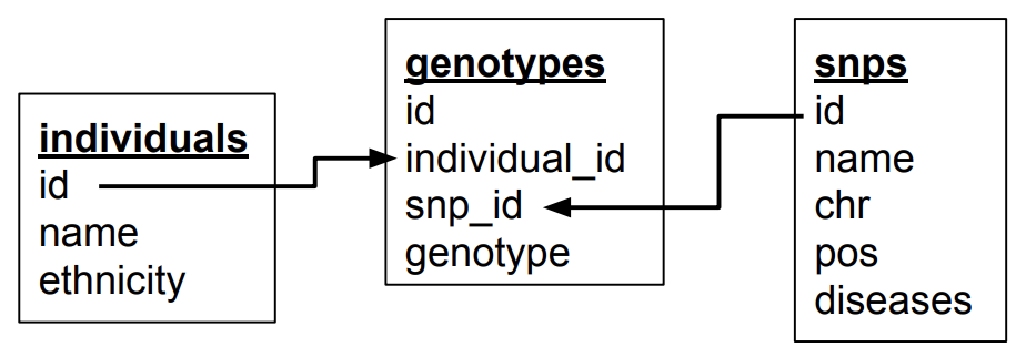
In the new table above, we see that there are several columns that are 1-to-1 dependent on another column. For example, if we know the individual, we know their ethnicity. If we know the SNP, we know the chromosome, position and any diseases involved. For the 2nd normal form, we extract these into separate tables. In doing this, think about the concepts that you’re trying to separate.
genotypes table:
| id | individual_id | snp_id | genotype |
|---|---|---|---|
1 |
1 |
1 |
A/A |
2 |
1 |
1 |
A/A |
3 |
2 |
1 |
A/C |
4 |
2 |
1 |
A/C |
5 |
1 |
2 |
A/G |
6 |
2 |
2 |
G/G |
7 |
1 |
3 |
G/T |
8 |
2 |
3 |
G/G |
individuals table:
| id | name | ethnicity |
|---|---|---|
1 |
individual_A |
caucasian |
2 |
individual_B |
caucasian |
snps table:
| id | name | chr | pos | diseases |
|---|---|---|---|---|
1 |
rs12345 |
1 |
12345 |
COPD |
2 |
rs12345 |
1 |
12345 |
asthma |
3 |
rs98765 |
1 |
98765 |
|
4 |
rs28465 |
5 |
28465 |
Some observations (and good practices):
-
The name of each table should be plural (not mandatory, but good practice).
-
Each table should have a primary key, ideally named
id. Different tables can contain columns that have the same name; column names should be unique within a table, but can occur across tables. -
In the
genotypestable, individuals are identified by theiridin theindividualstable which is their primary key. Theindividual_idcolumn in thegenotypestable is called the foreign key. Again best practice: if a foreign key refers to theidcolumn in theindividualstable, it should be namedindividual_id(note the singular). -
The name of each table should be plural (not mandatory, but good practice).
-
The foreign key
individual_idin thegenotypestable must be of the same type as theidcolumn in theindividualstable.
By the way, we see that the first 2 rows in the genotypes table are exactly the same apart from the unique ID, and the same is true for rows 3 and 4, so we can remove one for each (e.g. the ones with ID 2 and 4).
genotypes table:
| id | individual_id | snp_id | genotype |
|---|---|---|---|
1 |
1 |
1 |
A/A |
3 |
2 |
1 |
A/C |
5 |
1 |
2 |
A/G |
6 |
2 |
2 |
G/G |
7 |
1 |
3 |
G/T |
8 |
2 |
3 |
G/G |
The new schema:
Third normal form
-
Look for rows that are the same except for a non-key column
In the snps table above, there are two rows that are exactly the same (not taking into account the id column), if it weren’t for the disease field.
| 1 | rs12345 | 1 | 12345 | COPD |
|---|---|---|---|---|
2 |
rs12345 |
1 |
12345 |
asthma |
Such case indicates a one-to-many or many-to-many relationship: a single SNP can be involved in multiple diseases. Again we have duplication here: the fact that SNP rs12345 is on chromosome 1 at position 12345 is captured twice. We can solve this by extracting another table, called diseases.
Although biologically incorrect, imagine that a disease can only be linked to a single SNP. This would be a one-to-many relationship: one SNP to many diseases. In that case we could create the following tables:
snps table:
| id | name | chr | pos |
|---|---|---|---|
1 |
rs12345 |
1 |
12345 |
2 |
rs12345 |
1 |
12345 |
3 |
rs98765 |
1 |
98765 |
4 |
rs28465 |
5 |
28465 |
diseases table:
| id | name | snp_id |
|---|---|---|
1 |
COPD |
1 |
2 |
asthma |
1 |
We have now eliminated the disease column from the snps table so end up with 2 identical rows (rows 1 and 2) and can remove one of them.
| id | name | chr | pos |
|---|---|---|---|
1 |
rs12345 |
1 |
12345 |
2 |
rs12345 |
1 |
12345 |
3 |
rs98765 |
1 |
98765 |
4 |
rs28465 |
5 |
28465 |
But as we just mentioned, biologically speaking a single SNP can be involved in multiple diseases and a single disease can be influenced by multiple SNPs. This is a many-to-many relationship. In this case, we can’t just add a snp_id to the diseases table anymore (or you would have to use a non-atomic field which would violate the 1st normal form). You typically create a separate link table.
snps table:
| id | name | chr | pos |
|---|---|---|---|
1 |
rs12345 |
1 |
12345 |
3 |
rs98765 |
1 |
98765 |
4 |
rs28465 |
5 |
28465 |
diseases table:
| id | name |
|---|---|
1 |
COPD |
2 |
asthma |
disease2snp table:
| id | snp_id | disease_id |
|---|---|---|
1 |
1 |
1 |
2 |
1 |
2 |
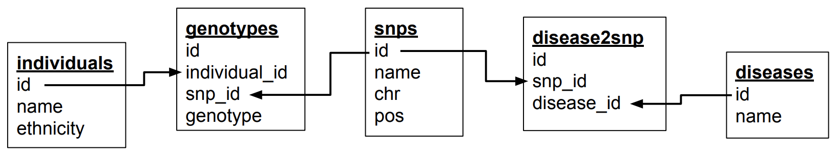
The final database
In the end, we have the following tables:
snps table:
| id | name | chr | pos |
|---|---|---|---|
1 |
rs12345 |
1 |
12345 |
2 |
rs98765 |
1 |
98765 |
3 |
rs28465 |
5 |
28465 |
diseases table:
| id | name |
|---|---|
1 |
COPD |
2 |
asthma |
disease2snp table:
| id | snp_id | disease_id |
|---|---|---|
1 |
1 |
1 |
2 |
1 |
2 |
genotypes table:
| id | individual_id | snp_id | genotype |
|---|---|---|---|
1 |
1 |
1 |
A/A |
3 |
2 |
1 |
A/C |
4 |
1 |
2 |
A/G |
5 |
2 |
2 |
G/G |
6 |
1 |
3 |
G/T |
7 |
2 |
3 |
G/G |
individuals table:
| id | name | ethnicity |
|---|---|---|
1 |
individual_A |
caucasian |
2 |
individual_B |
caucasian |
The schema itself:
Types of table relationships
To come back to the one-to-many relationships… So how do you know in which table to create the foreign key? Should there be an individual_id in the genotypes table? Or a genotype_id in the individuals table? That all depends on the type of relationship between two tables. This type can be:
-
one-to-one, for example an single ISBN number can be linked to a single book and vice versa.
-
one-to-many, for example a single company will have many employees, but a single employee will work only for a single company
-
many-to-many, for example a single book can have multiple authors and a single author can have written multiple books
One-to-many is obviously the same as many-to-one but looking at it from the other direction…
When you have a one-to-one relationship, you can actually merge that information into the same table so in the end you won’t even need a foreign key. In the book example mentioned above, you’d just add the ISBN number to the books table.
When you have a one-to-many relationship, you’d add the foreign key to the "many" table. In the example below a single company will have many employees, so you add the foreign key in the employees table.
The companies table:
| id | company_name |
|---|---|
1 |
Big company 1 |
2 |
Big company 2 |
3 |
Big company 3 |
… |
… |
The employees table:
| id | name | address | city | company_id |
|---|---|---|---|---|
1 |
John Jones |
some_address |
some_city |
1 |
2 |
Jim James |
another_address |
some_city |
1 |
3 |
Fred Fredricks |
yet_another_address |
another_city |
1 |
… |
… |
… |
… |
… |
When you have a many-to-many relationship you’d typically extract that information into a new table. For the books/authors example, you’d have a single table for the books, a single table for the authors, and a separate table that links the two together. That "linking" table can also contain information that is specific for that relationship, but it does not have to. An example is the genotypes table above. There are many SNPs for a single individual, and a single SNP is measured for many individuals. That’s why we created a separate table called genotypes, which in this case has additional columns that denote the value for a single individual for a single SNP. For the books/authors example, this would be:
The books table:
| id | title | ISBN13 |
|---|---|---|
1 |
Good Omens: The Nice and Accurate Prophecies of Agnes Nutter |
9780060853983 |
2 |
Going Postal (Discworld #33) |
9780060502935 |
3 |
Small Gods (Discworld #13) |
9780552152976 |
4 |
The Stupidest Angel: A Heartwarming Tale of Christmas Terror |
9780060842352 |
… |
… |
… |
The authors table:
| id | name |
|---|---|
1 |
Terry Pratchett |
2 |
Christopher Moore |
3 |
Neil Gaiman |
… |
… |
The author2book table:
| id | author_id | book_id |
|---|---|---|
1 |
1 |
1 |
2 |
3 |
1 |
3 |
1 |
2 |
4 |
1 |
3 |
5 |
2 |
4 |
… |
… |
… |
The information in these tables says that:
-
Terry Pratchett and Neil Gaiman co-wrote "Good Omens"
-
Terry Pratchett wrote "Going Postal" and "Small Gods" by himself
-
Christopher Moore was the single authors of "The Stupidest Angel"
1.3.4. Other best practices
There are some additional guidelines that you can use in creating your database schema, although different people use different guidelines. Everyone ends up with their own approach. What I do:
-
No capitals in table or column names
-
Every table name is plural (e.g.
genes) -
The primary key of each table should be
id -
Any foreign key should be the singular of the table name, plus "_id". So for example, a genotypes table can have a sample_id column which refers to the id column of the samples table.
In some cases, I digress from the rule of "every table name is plural", especially if a table is really meant to link to other tables together. A table genotypes which has an id, sample_id, snp_id, and genotype could e.g. also be called sample2snp.
1.3.5. Referential integrity
In a SQL database, it is important that there are no tables that contain a foreign key which cannot be resolved. For example in the genotypes table above, there should not be a row where the individual_id is 9 because there does not exist a record in the individuals table with an id of 9.
This might occur when you originally have that record in the individuals table, but removed it (either accidentally or on purpose). Large database management systems like Oracle actually will complain when you try to do that, and do not allow you to remove that row before any row referencing it in another table is removed first. As SQLite is lightweight, however, you will have to take care of this yourself.
This also means that when loading data, you should first load the individuals and snps tables, and only load the genotypes table afterwards, because the ids of the specific individuals and snps is otherwise not known yet.
1.3.6. Indices
There might be columns that you will often use for filtering. For example, you expect to regularly run queries that include a filter on ethnicity. To speed things up you can create an index on that column.
CREATE INDEX idx_ethnicity ON genotypes (ethnicity);1.4. SQL - Structured Query Language
Any interaction with data in RDBMS can happen through the Structured Query Language (SQL): create tables, insert data, search data, … There are two subparts of SQL:
DDL - Data Definition Language:
CREATE DATABASE test;
CREATE TABLE snps (id INT PRIMARY KEY AUTOINCREMENT, accession STRING, chromosome STRING, position INTEGER);
ALTER TABLE...
DROP TABLE snps;
For examples: see above.
DML - Data Manipulation Language:
SELECT
UPDATE
INSERT
DELETE
Some additional functions are:
DISTINCT
COUNT(*)
COUNT(DISTINCT column)
MAX(), MIN(), AVG()
GROUP BY
UNION, INTERSECT
We’ll look closer at getting data into a database and then querying it, using these four SQL commands.
1.4.1. Getting data in
INSERT INTO
There are several ways to load data into a database. The method used above is the most straightforward but inadequate if you have to load a large amount of data.
It’s basically:
INSERT INTO <table_name> (<column_1>, <column_2>, <column_3>)
                         VALUES (<value_1>, <value_2>, <value_3>);
Importing a datafile
But this becomes an issue if you have to load 1,000s of records. Luckily, it’s possible to load data from a comma-separated file straight into a table. Suppose you want to load 3 more individuals, but don’t want to type the insert commands straight into the sql prompt. Create a file (e.g. called data.csv) that looks like this:
individual_C,african
individual_D,african
individual_C,asian
Using DB Browser
Using the DB Browser, you can just go to File → Import → Table from CSV File…. Note that when you import a file like that, the system will automatically create the rowid column that will serve as the primary key.
On the command line
SQLite contains a .import command to load this type of data. Syntax: .import <file> <table>. So you could issue:
.separator ','
.import data.csv individualsAargh… We get an error!
Error: data.tsv line 1: expected 3 columns of data but found 2
This is because the table contains an ID column that is used as primary key and that increments automatically. Unfortunately, SQLite cannot work around this issue automatically. One option is to add the new IDs to the text file and import that new file. But we don’t want that, because it screws with some internal counters (SQLite keeps a counter whenever it autoincrements a column, but this counter is not adjusted if you hardwire the ID). A possible workaround is to create a temporary table (e.g. individuals_tmp) without the id column, import the data in that table, and then copy the data from that temporary table to the real individuals.
.schema individuals
CREATE TABLE individuals_tmp (name STRING, ethnicity STRING);
.separator ','
.import data.csv individuals_tmp
INSERT INTO individuals (name, ethnicity) SELECT * FROM individuals_tmp;
DROP TABLE individuals_tmp;
Your individuals table should now look like this (using SELECT * FROM individuals;):
| id | name | ethnicity |
|---|---|---|
1 |
individual_A |
caucasian |
2 |
individual_B |
caucasian |
3 |
individual_C |
african |
4 |
individual_D |
african |
5 |
individual_E |
asian |
1.4.2. Getting data out
It may seem counter-intuitive to first break down the data into multiple tables using the normal forms as described above, in order to having to combine them afterwards again in a SQL query. The reason for this is simple: it allows you to ask the data any question much more easily, instead of being restricted to the format of the original data.
Queries
Why do we need queries? Because natural languages (e.g. English) are too vague: with complex questions, it can be hard to verify that the question was interpreted correctly, and that the answer we received is truly correct. The Structured Query Language (SQL) is a standardised system so that users and developers can learn one method that works on (almost) any system.
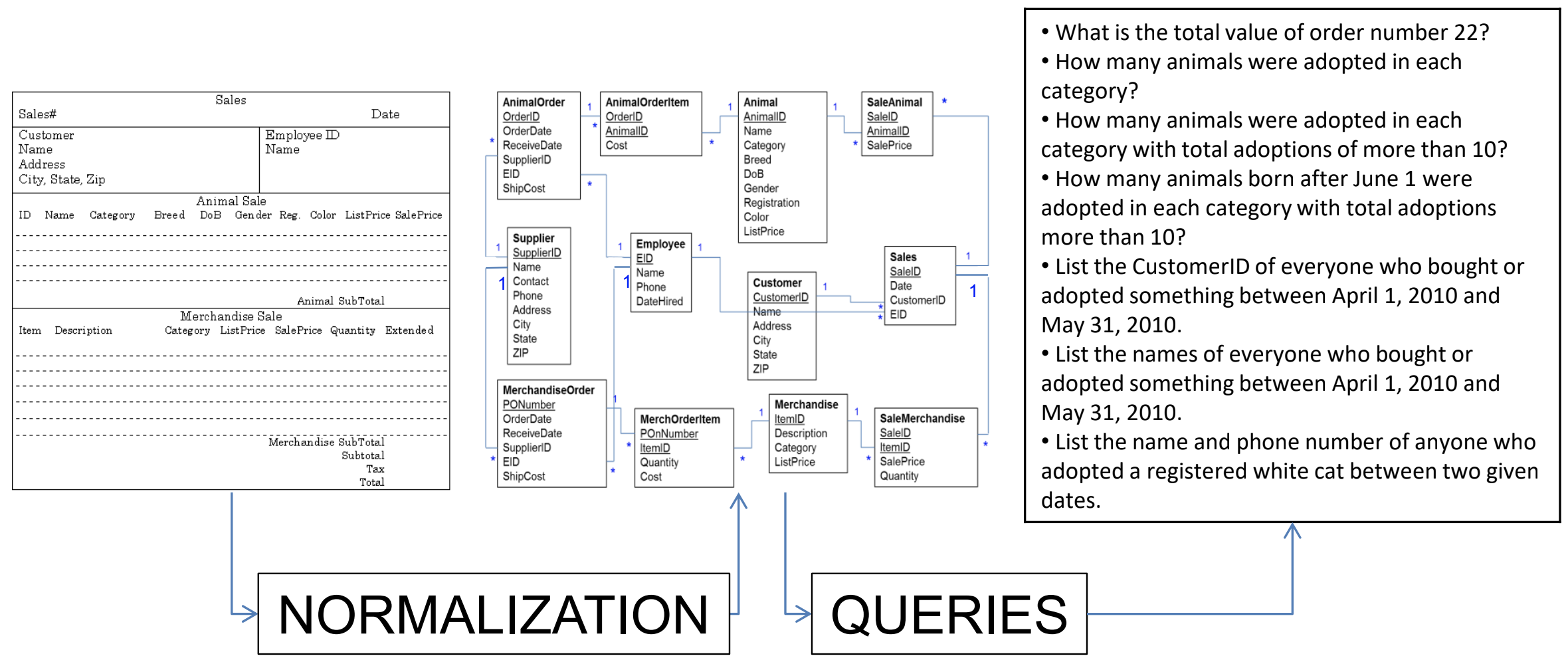
In order to write your queries, you’ll need to know what the database looks like. A relationship diagram including tables, columns and relations is very helpful here. See for example this relationship diagram for a pet store.
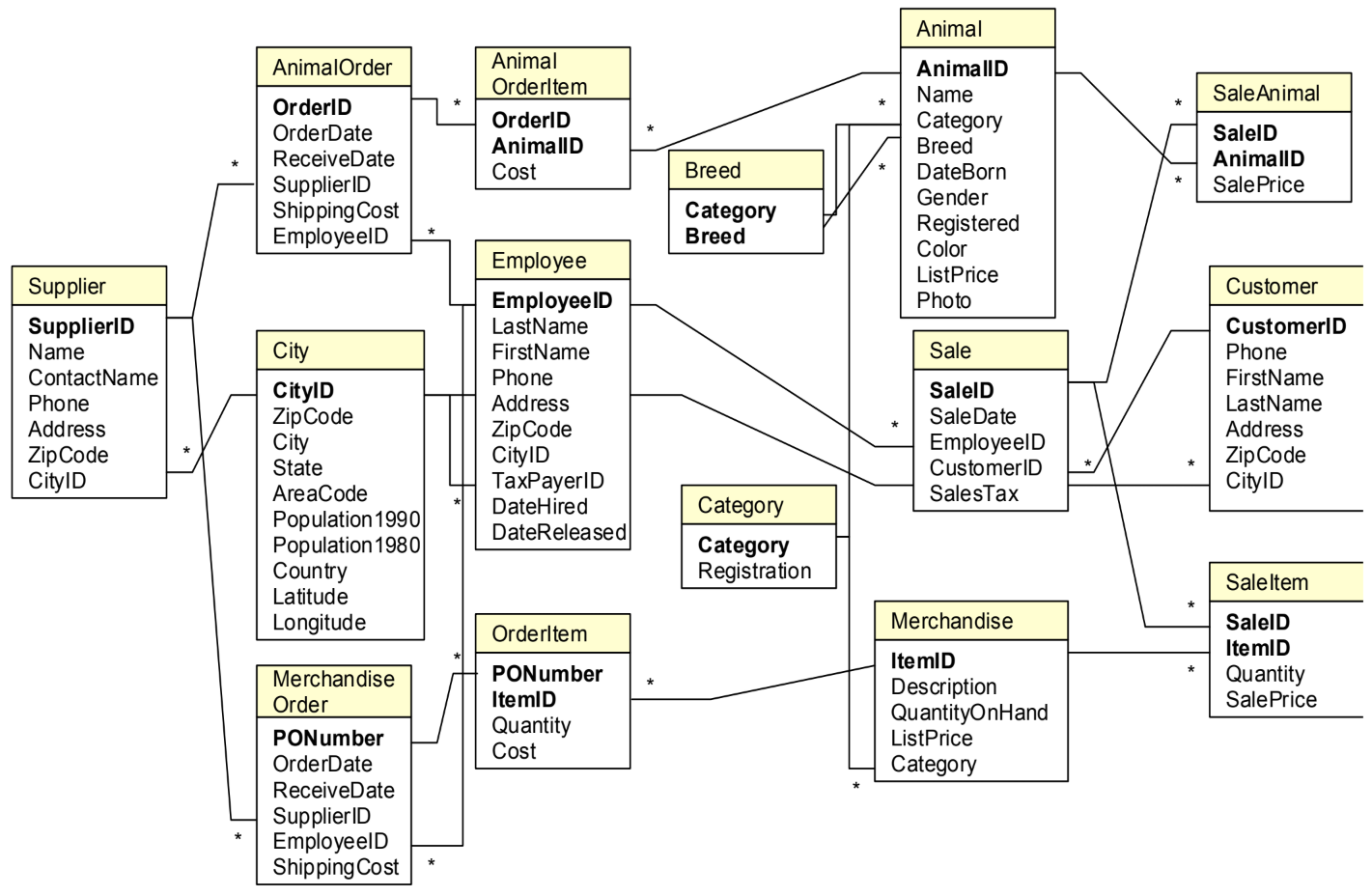
Questions that we can ask the database include:
-
Which animals were born after August 1?
-
List the animals by category and breed.
-
List the categories of animals that are in the Animal list.
-
Which dogs have a donation value greater than $250?
-
Which cats have black in their color?
-
List cats excluding those that are registered or have red in their color.
-
List all dogs who are male and registered or who were born before 01-June-2010 and have white in their color.
-
What is the extended value (price * quantity) for sale items on sale 24?
-
What is the average donation value for animals?
-
What is the total value of order number 22?
-
How many animals were adopted in each category?
-
How many animals were adopted in each category with total adoptions of more than 10?
-
How many animals born after June 1 were adopted in each category with total adoptions more than 10?
-
List the CustomerID of everyone who bought or adopted something between April 1, 2010 and May 31, 2010.
-
List the names of everyone who bought or adopted something between April 1, 2010 and May 31, 2010.
-
List the name and phone number of anyone who adopted a registered white cat between two given dates.
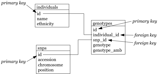
Similarly, we already drew the relationship diagram for the genotypes.
Questions that we can ask:
-
What is the number of individuals for each ethnicity?
-
How many SNPs are there per chromosome?
-
Approximately how long is chromosome 22 (by looking at the maximum SNP position)?
-
What are the most/least common genotypes?
-
…
Single tables
It is very simple to query a single table. The basic syntax is:
SELECT <column_name1, column_name2> FROM <table_name> WHERE <conditions>;If you want to see all columns, you can use "*" instead of a list of column names, and you can leave out the WHERE clause. The simplest query is therefore SELECT * FROM <table_name>;. So the <column_name1, column_name2> slices the table vertically while the WHERE clause slices it horizontally.
Data can be filtered using a WHERE clause. For example:
SELECT * FROM individuals WHERE ethnicity = 'african';
SELECT * FROM individuals WHERE ethnicity = 'african' OR ethnicity = 'caucasian';
SELECT * FROM individuals WHERE ethnicity IN ('african', 'caucasian');
SELECT * FROM individuals WHERE ethnicity != 'asian';
What if you can’t remember if the ethnicity was stored capitalised or not? In other words: was it 'caucasian' or 'Caucasian'? One way of approaching this is using the LIKE keyword. It behaves the same as ==, but you can use wildcards (i.c. %) that can represent any character. For example, the following two are almost the same:
SELECT * FROM individuals WHERE ethnicity == 'Caucasian' OR ethnicity == 'caucasian';
SELECT * FROm individuals WHERE ethnicity LIKE '%aucasian';
I say "almost" the same, because the % can stand for more than one character. A WHERE ethnicity LIKE '%sian' would therefore return those individuals who are "Caucasian", "caucasian", "Asian" and "asian".
You often just want to see a small subset of data just to make sure that you’re looking at the right thing. In that case: add a LIMIT clause to the end of your query, which has the same effect as using head on the linux command-line. Please always do this if you don’t know what your table looks like because you don’t want to send millions of lines to your screen.
SELECT * FROM individuals LIMIT 5;
SELECT * FROM individuals WHERE ethnicity = 'caucasian' LIMIT 1;
If you just want know the number of records that would match your query, use COUNT(*):
SELECT COUNT(*)
FROM individuals
WHERE ethnicity = 'african';
Using the GROUP BY clause you can aggregate data. For example:
SELECT ethnicity, COUNT(*)
FROM individuals
GROUP BY ethnicity;
======= Combining tables
In the second normal form we separated several aspects of the data in different tables. Ultimately, we want to combine that information of course. This is where the primary and foreign keys come in. Suppose you want to list all different SNPs, with the alleles that have been found in the population:
SELECT individual_id, snp_id, genotype_amb
FROM genotypes;
This isn’t very informative, because we get the uninformative numbers for SNPs instead of SNP accession numbers. To run a query across tables, we have to call both tables in the FROM clause:
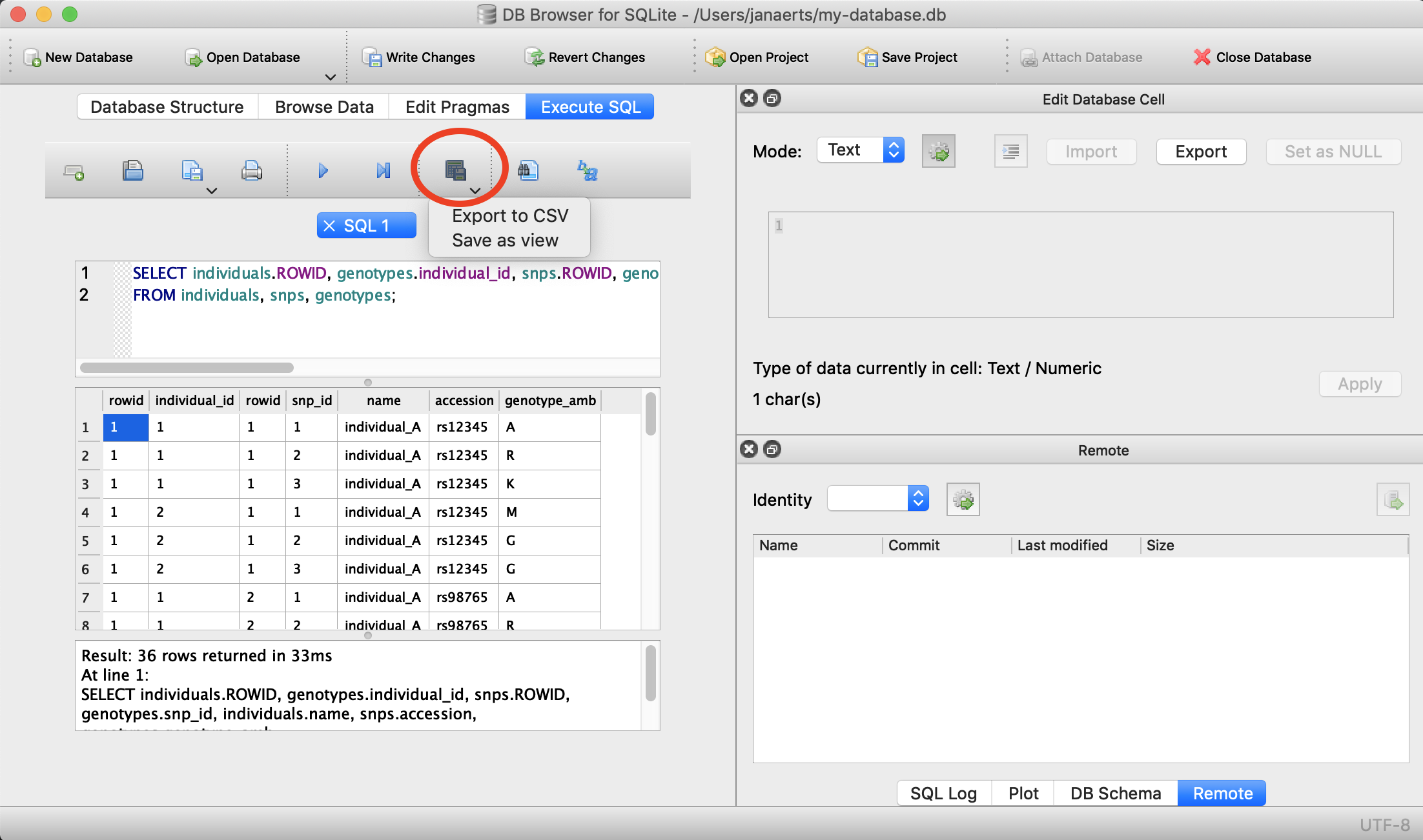
SELECT individuals.name, snps.accession, genotypes.genotype_amb
FROM individuals, snps, genotypes;| name | accession | genotype_amb |
|---|---|---|
individual_A |
rs12345 |
A |
individual_A |
rs12345 |
R |
individual_A |
rs12345 |
K |
individual_A |
rs12345 |
M |
individual_A |
rs12345 |
G |
individual_A |
rs12345 |
G |
individual_A |
rs98765 |
A |
individual_A |
rs98765 |
R |
individual_A |
rs98765 |
K |
individual_A |
rs98765 |
M |
individual_A |
rs98765 |
G |
individual_A |
rs98765 |
G |
individual_A |
rs28465 |
A |
individual_A |
rs28465 |
R |
individual_A |
rs28465 |
K |
individual_A |
rs28465 |
M |
individual_A |
rs28465 |
G |
individual_A |
rs28465 |
G |
individual_B |
rs12345 |
A |
individual_B |
rs12345 |
R |
individual_B |
rs12345 |
K |
individual_B |
rs12345 |
M |
individual_B |
rs12345 |
G |
individual_B |
rs12345 |
G |
individual_B |
rs98765 |
A |
individual_B |
rs98765 |
R |
individual_B |
rs98765 |
K |
individual_B |
rs98765 |
M |
individual_B |
rs98765 |
G |
individual_B |
rs98765 |
G |
individual_B |
rs28465 |
A |
individual_B |
rs28465 |
R |
individual_B |
rs28465 |
K |
individual_B |
rs28465 |
M |
individual_B |
rs28465 |
G |
individual_B |
rs28465 |
G |
Wait… This can’t be correct: we get 36 rows back instead of the 6 that we expected. This is because all combinations are made between all rows of each table. We have to put some constraints on the rows that are returned.
SELECT individuals.name, snps.accession, genotypes.genotype_amb
FROM individuals, snps, genotypes
WHERE individuals.id = genotypes.individual_id
AND snps.id = genotypes.snp_id;| name | accession | genotype_amb |
|---|---|---|
individual_A |
rs12345 |
A |
individual_A |
rs98765 |
R |
individual_A |
rs28465 |
K |
individual_B |
rs12345 |
M |
individual_B |
rs98765 |
G |
individual_B |
rs28465 |
G |
What happens here?
-
The individuals, snps and genotypes tables are referenced in the FROM clause.
-
In the SELECT clause, we tell the query what columns to return. We prepend the column names with the table name, to know what column we actually mean (snps.id is a different column from individuals.id).
-
In the WHERE clause, we actually provide the link between the tables: the value for snp_id in the genotypes table should correspond with the id column in the snps table. This is the part that solves the above issue of returning all those nonsense rows. Imagine that we’d ask the id’s themselves as well, then we’d get the list below. From that list, we can then filter the rows that adhere to the constraints we set.
SELECT individuals.id, genotypes.individual_id, snps.id, genotypes.snp_id, individuals.name, snps.accession, genotypes.genotype_amb
FROM individuals, snps, genotypes;| individual.id | genotypes.individual_id | snps.id | genotypes.snp_id | name | accession | genotype_amb |
|---|---|---|---|---|---|---|
1 |
1 |
1 |
1 |
individual_A |
rs12345 |
A |
1 |
1 |
-1- |
-2- |
individual_A |
rs12345 |
R |
1 |
1 |
-1- |
-3- |
individual_A |
rs12345 |
K |
-1- |
-2- |
1 |
1 |
individual_A |
rs12345 |
M |
-1- |
-2- |
-1- |
-2- |
individual_A |
rs12345 |
G |
-1- |
-2- |
-1- |
-3- |
individual_A |
rs12345 |
G |
1 |
1 |
-2- |
-1- |
individual_A |
rs98765 |
A |
1 |
1 |
2 |
2 |
individual_A |
rs98765 |
R |
1 |
1 |
-2- |
-3- |
individual_A |
rs98765 |
K |
-1- |
-2- |
-2- |
-1- |
individual_A |
rs98765 |
M |
-1- |
-2- |
2 |
2 |
individual_A |
rs98765 |
G |
-1- |
-2- |
-2- |
-3- |
individual_A |
rs98765 |
G |
1 |
1 |
-3- |
-1- |
individual_A |
rs28465 |
A |
1 |
1 |
-3- |
-2- |
individual_A |
rs28465 |
R |
1 |
1 |
3 |
3 |
individual_A |
rs28465 |
K |
-1- |
-2- |
-3- |
-1- |
individual_A |
rs28465 |
M |
-1- |
-2- |
-3- |
-2- |
individual_A |
rs28465 |
G |
-1- |
-2- |
3 |
3 |
individual_A |
rs28465 |
G |
-2- |
-1- |
1 |
1 |
individual_B |
rs12345 |
A |
-2- |
-1- |
-1- |
-2- |
individual_B |
rs12345 |
R |
-2- |
-1- |
-1- |
-3- |
individual_B |
rs12345 |
K |
2 |
2 |
1 |
1 |
individual_B |
rs12345 |
M |
… |
… |
… |
… |
… |
… |
… |
Having to type the table names in front of the column names can become tiresome. We can however create aliases like this:
SELECT i.name, s.accession, g.genotype_amb
FROM individuals i, snps s, genotypes g
WHERE i.id = g.individual_id
AND s.id = g.snp_id;
JOIN
Sometimes, though, we have to join tables in a different way. Suppose that our snps table contains SNPs that are nowhere mentioned in the genotypes table, but we still want to have them mentioned in our output:
INSERT INTO snps (accession, chromosome, position) VALUES ('rs11223','2',11223);If we run the following query:
SELECT s.accession, s.chromosome, s.position, g.genotype_amb
FROM snps s, genotypes g
WHERE s.id = g.snp_id
ORDER BY s.accession, g.genotype_amb;
We get the following output:
| chromosome | position | accession | genotype_amb |
|---|---|---|---|
1 |
12345 |
rs12345 |
A |
1 |
12345 |
rs12345 |
M |
1 |
98765 |
rs98765 |
G |
1 |
98765 |
rs98765 |
R |
5 |
28465 |
rs28465 |
G |
5 |
28465 |
rs28465 |
K |
But we actually want to have rs11223 in the list as well. Using this approach, we can’t because of the WHERE s.id = g.snp_id clause. The solution to this is to use an explicit join. To make things complicated, there are several types: inner and outer joins. In principle, an inner join gives the result of the intersect between two tables, while an outer join gives the results of the union. What we’ve been doing up to now is look at the intersection, so the approach we used above is equivalent to an inner join:
SELECT s.accession, g.genotype_amb
FROM snps s INNER JOIN genotypes g ON s.id = g.snp_id
ORDER BY s.accession, g.genotype_amb;
gives:
| accession | genotype_amb |
|---|---|
rs12345 |
A |
rs12345 |
M |
rs28465 |
G |
rs28465 |
K |
rs98765 |
G |
rs98765 |
R |
A left outer join returns all records from the left table, and will include any matches from the right table:
SELECT s.accession, g.genotype_amb
FROM snps s LEFT OUTER JOIN genotypes g ON s.id = g.snp_id
ORDER BY s.accession, g.genotype_amb;
gives:
| accession | genotype_amb |
|---|---|
rs11223 |
|
rs12345 |
A |
rs12345 |
M |
rs28465 |
G |
rs28465 |
K |
rs98765 |
G |
rs98765 |
R |
(Notice the extra line for rs11223!)
A full outer join, finally, return all rows from the left table, and all rows from the right table, matching any rows that should be.
Export to file
Often you will want to export the output you get from an SQL-query to a file (e.g. CSV) on your operating system so that you can use that data for external analysis in R or for visualisation. This is easy to do. Suppose that we want to export the first 5 lines of the snps table into a file called 5_snps.csv.
Using DB Browser
There’s a button for that…
On the command line
You do that like this:
.header on
.mode csv
.once 5_snps.csv
SELECT * FROM snps LIMIT 5;
If you now exit the sqlite prompt (with .quit), you should see a file in the directory where you were that is called 5_snps.csv.
1.4.3. Updating and deleting data
Sometimes you will want to update or delete data in a table. The SQL code to do this uses a WHERE clause that is exactly the same as for a regular SELECT.
|
Tip
|
First do a SELECT on your table with the WHERE clause that you’ll use for the update or deletion just to make sure that you’ll change the correct rows. When you’ve made changes to the wrong rows you won’t be able to go back (unless you use the Lambda architecture principles as we will explain in the third session).
|
UPDATE
Imagine that we’ve been storing the information on our individuals as above, but have not been consistent in capitalising the ethnicity. In some cases, a person can be of asian descent; in other cases he or she can be Asian. The same would go for the other ethnicities. To clean this up, let’s put everything in lower case. For argument’s sake we’ll only look at Asian here. First let’s check what we should get with a SELECT.
SELECT * FROM individuals
WHERE ethnicity == 'Asian';
This will give us the rows that we will change. Are these indeed the ones? Then go forward with the update:
UPDATE individuals
SET ethnicity = 'asian'
WHERE ethnicity == 'Asian';
The WHERE clause is the same. The general syntax for an update looks like this:
UPDATE <table>
SET <column> = <new value>
WHERE <conditions>;
In this example the column that is updated (ethnicity) is the same as the one in the WHERE clause. This does not have to be the case. What would the following do?
UPDATE genotypes
SET genotype_amb = 'R'
WHERE genotype == 'A/G';
DELETE
DELETE is similar to UPDATE but simpler: you don’t use the SET pragma. Same as with updating data, make sure that your WHERE clause is correct! Test this with a SELECT beforehand.
The general syntax:
DELETE FROM <table>
WHERE <conditions>;
For example:
DELETE FROM genotypes
WHERE genotype_amb == 'N';
1.4.4. Additional functions
LIMIT
If you only want to get the first 10 results back (e.g. to find out if your complicated query does what it should do without running the whole actual query), use LIMIT:
sqlite> SELECT * FROM snps LIMIT 2;NULL
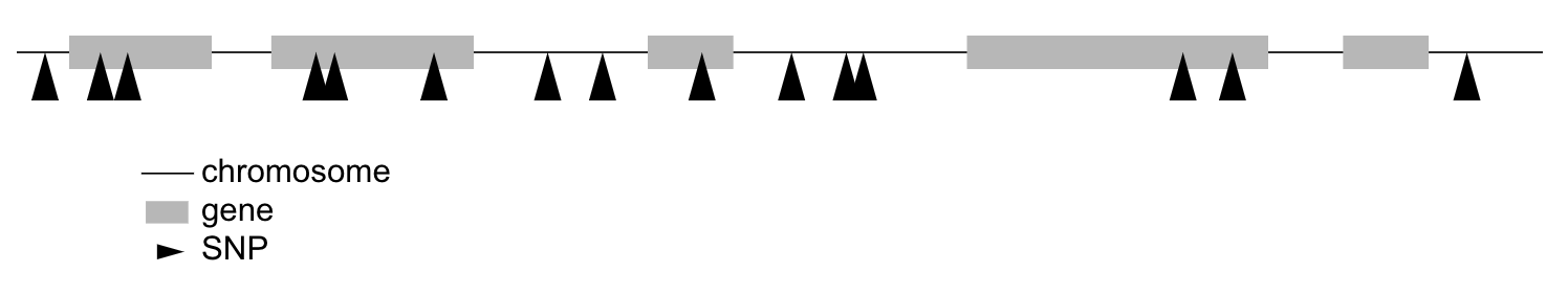
SNPs are spread across a chromosome, and might or might not be located within a gene.
What if you want to search for the SNPs that are not in genes? Imagine that our snps table has an additional column with the gene name, like this:
| id | accession | chromosome | position | gene |
|---|---|---|---|---|
1 |
rs12345 |
1 |
12345 |
gene_A |
2 |
rs98765 |
1 |
98765 |
gene_A |
3 |
rs28465 |
5 |
28465 |
gene_B |
4 |
rs92873 |
7 |
7382 |
|
5 |
rs10238 |
11 |
291732 |
gene_C |
6 |
rs92731 |
17 |
10283 |
gene_C |
We cannot SELECT * FROM snps WHERE gene = ""; because that is searching for an empty string which is not the same as a missing value. To get to rs92873 you can issue SELECT * FROM snps WHERE gene IS NULL; or to get the rest SELECT * FROM snps WHERE GENE IS NOT NULL;. Note that it is IS NULL and not = NULL…
AND, OR
Your queries might need to combine different conditions, as we’ve already seen above:
-
AND: both must be true -
OR: either one is true -
NOT: reverse the value
SELECT * FROM snps WHERE chromosome = '1' AND position < 40000;
SELECT * FROM snps WHERE chromosome = '1' OR chromosome = '5';
SELECT * FROM snps WHERE chromosome = '1' AND NOT position < 40000;
The result is affected by the order of the operations. Parentheses indicate that an operation should be performed first. Without parentheses, operations are performed left-to-right.
For example, if a = 3, b = -1 and c = 2, then:
-
(( a > 4 ) AND ( b < 0 )) OR ( c > 1 ) evaluates to true
-
( a > 4 ) AND (( b < 0 ) OR ( c > 1 )) evaluates to false
De Morgan’s laws apply to SQL. The rules allow the expression of conjunctions and disjunctions purely in terms of each other via negation. For example:
-
NOT (A AND B)becomesNOT A OR NOT B -
NOT (A OR B)becomesNOT A AND NOT B
IN
The IN clause defines a set of values. It is a shortcut to combine several entries with an OR condition.
For example, instead of writing
SELECT *
FROM customer
WHERE first_name = 'Tim'
    OR first_name = 'David'
    OR first_name = 'Jay';
you can use
SELECT *
FROM customer
WHERE first_name IN ('Tim', 'David', 'Jay');
DISTINCT
Whenever you want the unique values in a column: use DISTINCT in the SELECT clause:
SELECT category FROM animal;| category |
|---|
Fish |
Dog |
Fish |
Cat |
Cat |
Dog |
Fish |
Dog |
Dog |
Dog |
Fish |
Cat |
Dog |
… |
SELECT DISTINCT category FROM animal;| distinct(category) |
|---|
Bird |
Cat |
Dog |
Fish |
Mammal |
Reptile |
Spider |
DISTINCT automatically sorts the results.
ORDER BY
The order by clause allows you to, well, order your output. By default, this is in ascending order. To order from large to small, you can add the DESC tag. It is possible to order by multiple columns, for example first by chromosome and then by position:
SELECT * FROM snps ORDER BY chromosome;
SELECT * FROM snps ORDER BY accession DESC;
SELECT * FROM snps ORDER BY chromsome, position;
COUNT
For when you want to count things:
SELECT COUNT(*) FROM genotypes WHERE genotype_amb = 'G';MAX(), MIN(), AVG()
…act as you would expect (only works with numbers, obviously):
SELECT MAX(position) FROM snps;Output is:
| max(position) |
|---|
291732 |
AS
In some cases you might want to rename the output column name. For instance, in the example above you might want to have maximum_position instead of max(position). The AS keyword can help us with that.
SELECT MAX(position) AS maximum_position FROM snps;GROUP BY
GROUP BY can be very useful in that it first aggregates data. It is often used together with COUNT, MAX, MIN or AVG:
SELECT genotype_amb, COUNT(*)
FROM genotypes
GROUP BY genotype_amb;

SELECT genotype_amb, COUNT(*) AS c
FROM genotypes
GROUP BY genotype_amb
ORDER BY c DESC;| genotype_amb | c |
|---|---|
G |
2 |
A |
1 |
K |
1 |
M |
1 |
R |
1 |
SELECT chromosome, MAX(position)
FROM snps
GROUP BY chromosome
ORDER BY chromosome;| chromosome | MAX(position) |
|---|---|
1 |
98765 |
2 |
11223 |
5 |
28465 |
HAVING
Whereas the WHERE clause puts conditions on certain columns, the HAVING clause puts these on groups created by GROUP BY.
For example, given the following snps table:
| id | accession | chromosome | position | gene |
|---|---|---|---|---|
1 |
rs12345 |
1 |
12345 |
gene_A |
2 |
rs98765 |
1 |
98765 |
gene_A |
3 |
rs28465 |
5 |
28465 |
gene_B |
4 |
rs92873 |
7 |
7382 |
|
5 |
rs10238 |
11 |
291732 |
gene_C |
6 |
rs92731 |
17 |
10283 |
gene_C |
SELECT chromosome, count(*) as c
FROM snps
GROUP BY chromosome;
will return
| chromosome | c |
|---|---|
1 |
2 |
5 |
1 |
7 |
1 |
11 |
1 |
17 |
1 |
whereas
SELECT chromosome, count(*) as c
FROM snps
GROUP BY chromosome
HAVING c > 1
will return
| chromosome | c |
|---|---|
1 |
2 |
The HAVING clause must follow a GROUP BY, and precede a possible ORDER BY.
UNION, INTERSECT
It is sometimes hard to get the exact rows back that you need using the WHERE clause. In such cases, it might be possible to construct the output based on taking the union or intersection of two or more different queries:
SELECT * FROM snps WHERE chromosome = '1';
SELECT * FROM snps WHERE position < 40000;
SELECT * FROM snps WHERE chromosome = '1' INTERSECT SELECT * FROM snps WHERE position < 40000;| id | accession | chromosome | position |
|---|---|---|---|
1 |
rs12345 |
1 |
12345 |
LIKE
Sometimes you want to make fuzzy matches. What if you’re not sure if the ethnicity has a capital or not?
SELECT * FROM individuals WHERE ethnicity = 'African';returns no results…
SELECT * FROM individuals WHERE ethnicity LIKE '%frican';Note that different databases use different characters as wildcard. For example: % is a wildcard for MS SQL Server representing any string, and * is the corresponding wildcard character used in MS Access. Check the documentation for the RDBMS that you’re using (sqlite, MySQL/MariaDB, MS SQL Server, MS Access, Oracle, …) for specifics.
Subqueries
As we mentioned in the beginning, the general setup of a SELECT is:
SELECT <column_names>
FROM <table>
WHERE <condition>;
But as you’ve seen in the examples above, the output from any SQL query is itself basically a table. So we can actually use that output table to run another SELECT. For example:
SELECT *
FROM (
       SELECT *
       FROM snps
       WHERE chromosome IN ('1','5'))
WHERE position < 40000;
Of course, you can use UNION and INTERSECT in the subquery as well…
Another example:
SELECT COUNT(*)
FROM (
       SELECT DISTINCT genotype_amb
       FROM genotypes);
1.4.5. Public bioinformatics databases
Sqlite is a light-weight system for running relational databases. If you want to make your data available to other people it’s often better to use systems such as MySQL. The data behind the Ensembl and UCSC genome browsers, for example, is stored in a relational database and directly accessible through SQL as well.
If you install a mysql client (see www.mariadb.org or www.mysql.com), you can access these public databases as well. Another option is to run mysql using docker.
To access the last release of human from Ensembl: mysql -h ensembldb.ensembl.org -P 5306 -u anonymous homo_sapiens_core_70_37. To get an overview of the tables that we can query: show tables. Using docker this would be docker run -it --rm mysql mysql -h ensembldb.ensembl.org -u anonymous -P 5306 homo_sapiens_core_70_37.
To access the hg38 release of the UCSC database (which is also a MySQL database): mysql -h genome-mysql.soe.ucsc.edu -ugenome -A hg38. With docker: docker run -it --rm mysql mysql -h genome-mysql.soe.ucsc.edu -u genome -A hg38. You can then for example find out where the gene CYP3A4 is located with
SELECT name, name2, chrom, strand, txStart, txEnd, cdsStart, cdsEnd
FROM refGene
WHERE name2 = 'CYP3A4';
Output will be:
mysql> SELECT name, name2, chrom, strand, txStart, txEnd, cdsStart, cdsEnd
    -> FROM refGene
    -> WHERE name2 = 'CYP3A4';
+--------------+--------+-------+--------+----------+----------+----------+----------+
name, name2, chrom, strand, txStart, txEnd, cdsStart, cdsEnd
+--------------+--------+-------+--------+----------+----------+----------+----------+
NM_001202855, CYP3A4, chr7, -, 99756966, 99784184, 99758132, 99784081
NM_017460, CYP3A4, chr7, -, 99756966, 99784184, 99758132, 99784081
+--------------+--------+-------+--------+----------+----------+----------+----------+
2 rows in set (0.16 sec)
Note: Installing the complete mysql system will install the server and client, and it can be difficult to remove if necessary afterwards. An alternative is to install it using docker. Run the server with docker run --name some-mysql -e MYSQL_ROOT_PASSWORD=my-secret-pw -d mysql:latest and connect to it using docker exec -it some-mysql bash. You can then access the Ensembl and UCSC databases as described above.
1.4.6. Views
By decomposing data into different tables as we described above (and using the different normal forms), we can significantly improve maintainability of our database and make sure that it does not contain inconsistencies. But at the other hand, this means it’s a lot of hassle to look at the actual data: to know what the genotype is for SNP rs12345 in individual_A we cannot just look it up in a single table, but have to write a complicated query which joins 3 tables together. The query would look like this:
SELECT i.name, i.ethnicity, s.accession, s.chromosome, s.position, g.genotype_amb
FROM individuals i, snps s, genotypes g
WHERE i.id = g.individual_id
AND s.id = g.snp_id;
Output looks like this:
| name | ethnicity | accession | chromosome | position | genotype_amb |
|---|---|---|---|---|---|
individual_A |
caucasian |
rs12345 |
1 |
12345 |
A |
individual_A |
caucasian |
rs98765 |
1 |
98765 |
R |
individual_A |
caucasian |
rs28465 |
5 |
28465 |
K |
individual_B |
caucasian |
rs12345 |
1 |
12345 |
M |
individual_B |
caucasian |
rs98765 |
1 |
98765 |
G |
individual_B |
caucasian |
rs28465 |
5 |
28465 |
G |
There is however a way to make this easier: you can create views on the data. This basically saves the whole query and gives it a name. You do this by adding CREATE VIEW some_name AS to the front of the query, like this:
CREATE VIEW v_genotypes AS
SELECT i.name, i.ethnicity, s.accession, s.chromosome, s.position, g.genotype_amb
FROM individuals i, snps s, genotypes g
WHERE i.id = g.individual_id
AND s.id = g.snp_id;
You can think of this as if you had made a new table with the name v_genotypes that you can use just like any other table, for example:
SELECT *
FROM v_genotypes g
WHERE g.genotype_amb = 'R';
The difference with an actual table is, however, that the result of the view is actually not stored itself. Whenever you do SELECT * FROM v_genotypes, it will actually perform the whole query in the background.
Note: to make sure that I can tell by the name if something is a table or a view, I always add a v_ in front of the name that I give to the view.
Pivot tables
In some cases, you want to violate the 1st normal form, and have different columns represent the same type of data. A typical example is when you want to analyze your data in R using a dataframe. Let’s say we have expression values for different genes in different individuals. Being good programmers, we saved this data in the database like this:
| individual | gene | expression |
|---|---|---|
individual_A |
gene_A |
2819 |
individual_A |
gene_B |
1028 |
individual_A |
gene_C |
3827 |
individual_B |
gene_A |
1928 |
individual_B |
gene_B |
999 |
individual_B |
gene_C |
1992 |
In R, you will however probably want a dataframe that looks like this:
| gene | individual_A | individual_B |
|---|---|---|
gene_A |
2819 |
1928 |
gene_B |
1028 |
999 |
gene_C |
3827 |
1992 |
This is called a pivot table, and there are several ways to create these in SQLite. The method presented here is taken from http://bduggan.github.io/virtual-pivot-tables-opensqlcamp2009-talk/. To create such table (and store it in a view), you have to use group_concat and group_by:
CREATE VIEW v_pivot_expressions AS
SELECT gene,
       GROUP_CONCAT(CASE WHEN individual = 'individual_A' THEN expression ELSE NULL END) AS individual_A,
       GROUP_CONCAT(CASE WHEN individual = 'individual_B' THEN expression ELSE NULL END) AS individual_B
FROM expressions
GROUP BY gene;
1.5. Drawbacks of relational databases
Relational databases are great. They can be a big help in storing and organizing your data. But they are not the ideal solution in all situations.
1.5.1. Scalability
Relational databases are only scalable in a limited way. The fact that you try to normalise your data means that your data is distributed over different tables. Any query on that data often requires extensive joins. This is OK, until you have tables with millions of rows. A join can in that case a very long time to run.
[Although outside of the scope of this lecture.] One solution sometimes used is to go for a star-schema rather than a fully normalised schema. Or using a NoSQL database management system that is horizontally scalable (document-oriented, column-oriented or graph databases).
1.5.2. Modeling
Some types of information are difficult to model when using a relational paradigm. In a relational database, different records can be linked across tables using foreign keys. If you’re however really interested in the relations themselved (e.g. social graphs, protein-protein-interaction, …) you are much better of to use a real graph database (e.g. neo4j) instead of a relational database. In a graph database finding all neighbours-of-neighbours in a graph of 50 members (basically) takes as long as in a graph with 50 million members.
1.5.3. Drawback exercise
Suppose you want to model a social graph. People have names, and know other people. Every "know" is reciprocal (so if I know you then you know me). The data might look like this:
Tim knows Terry
Tom knows Terry
Terry knows Gerry
Gerry knows Rik
Gerry knows James
James knows John
Fred knows James
Frits knows Fred
In table format:
| knower | knowee |
|---|---|
Tim |
Terry |
Tom |
Terry |
Terry |
Gerry |
Gerry |
Rik |
Gerry |
James |
James |
John |
Fred |
James |
Frits |
Fred |
Gerry |
Frits |
If you really want to have this in a relational database, how would you find out who are the friends of the friends of James? First, we’d need to find out who James' friends are:
SELECT knower FROM friends WHERE knowee = 'James'
UNION
SELECT knowee FROM friends WHERE knower = 'James';
Using this as a subquery, we can then find out who the friends of those friends are:
SELECT knower FROM friends
WHERE knowee IN (
  SELECT knower FROM friends WHERE knowee = 'James'
  UNION
  SELECT knowee FROM friends WHERE knower = 'James'
)
UNION
SELECT knowee FROM friends
WHERE knower IN (
  SELECT knower FROM friends WHERE knowee = 'James'
  UNION
  SELECT knowee FROM friends WHERE knower = 'James'
);
If we want to know how big the group is, we’ll have to nest this again as a subquery:
SELECT COUNT(*) FROM (
  SELECT knower FROM friends
  WHERE knowee IN (
    SELECT knower FROM friends WHERE knowee = 'James'
    UNION
    SELECT knowee FROM friends WHERE knower = 'James'
  )
  UNION
  SELECT knowee FROM friends
  WHERE knower IN (
    SELECT knower FROM friends WHERE knowee = 'James'
    UNION
    SELECT knowee FROM friends WHERE knower = 'James'
  )
);
You can imagine that there must be better ways of doing this. Remember this example when you’ll learn about graph databases…
1.6. Python API to sqlite
To access sqlite databases from python, you can use the sqlite3 library, available here. See the this site for documentation on how to use the library.
Example use:
import sqlite3
connection = sqlite3.connect("tutorial.db")
cursor = connection.cursor()

for row in cur.execute("SELECT year, title FROM movie ORDER BY year"):
    print(row)