Parameter sensitivity
Are k-MSTs less sensitive to k than k-NNs? Intuitively the answer is yes because k-MSTs always produce a single connected component for every value of k. That is not always the case for k-NNs.
A better question asks how k influences dimensionality reduction performance. This notebook performs a parameter sensitivity analysis measuring how the sortedness metric changes for small changes in k: \(\Delta k\)
[ ]:
import numba
import warnings
import numpy as np
import pandas as pd
import lensed_umap as lu
from tqdm import tqdm
from itertools import product
from collections import defaultdict
from scipy.stats import weightedtau
from scipy.spatial.distance import cdist

from umap import UMAP
from multi_mst import KMSTDescent

from lib.data import get_datasets
from lib.plotting import *

_ = configure_matplotlib()
Datasets
We use a set of smaller real-world datasets to evaluate the algorithms because the sortedness measure has a quadratic computational complexity. These datasets have been used to evaluate clustering algorithms by campello et al., 2015 and Castro et al., 2019.
This repository includes code and/or instructions to download the datasets. See the respective notebooks/data/[dataset]/README.md file for instructions. The datasets that have been downloaded and/or pre-processed following those instructions are used.
[2]:
small_data_config = {
  key: loader
  for key, loader in  get_datasets().items()
  if loader().shape[0] < 10000
}
print(small_data_config.keys())
dict_keys(['iris', 'diabetes', 'wine', 'articles_1442_5', 'articles_1442_80', 'authorship', 'cardiotocography', 'cell_cycle_237', 'ecoli', 'elegans', 'horse', 'mfeat_factors', 'mfeat_karhunen', 'semeion', 'yeast_galactose'])
Parameter sweep
This section implements the parameter sensitivity analysis. First, we need a function to compute k-NN and k-MST graphs and their UMAP embeddings given a dataset and k.
[4]:
def compute_embedding(data, k, alg):
    with warnings.catch_warnings():
        warnings.simplefilter("ignore", category=UserWarning)
        warnings.simplefilter("ignore", category=FutureWarning)
        if alg == "kmst":
            p = (
                KMSTDescent(num_neighbors=k, metric="cosine")
                .fit(data)
                .umap(transform_mode="graph")
            )
        elif alg == "umap":
            p = UMAP(
                n_neighbors=k, force_approximation_algorithm=True, metric="cosine"
            ).fit(data, transform_mode="graph")
        p = lu.embed_graph(p, repulsion_strengths=[0.001, 0.01, 0.1, 1])
    return p.embedding_, p.graph_
Second, we need a function that computes the sortedness measure, comparing distance ranks between the raw data and the embedding:
[5]:
@numba.njit(parallel=True)
def rank_along_col(orders):
    """Convert per-row argsort order into ranks."""
    out = np.empty(orders.shape, dtype=np.intp)
    for row in numba.prange(orders.shape[0]):
        for i, o in enumerate(orders[row, :]):
            out[row, o] = i
    return out


def score_ranks(a, b):
    """Computes Sortedness from data ranks (a) and embedding ranks (b)."""
    sortedness = np.empty(a.shape[0], dtype=np.float32)
    for idx in range(a.shape[0]):
        sortedness[idx] = weightedtau(a[idx, :], b[idx, :], rank=a[idx, :]).statistic
    return np.mean(sortedness)
Finally, we need to evaluate both algorithms on the datasets at multiple values of k. Here, we select random values in 10 uniform segments on \(k = [2, 100]\). Each sampled value also gets perturbed with \(\pm \Delta k \in [2, 5, 10]\), randomly selecting the positive or negative direction. The resulting unique values for \(k\) are evaluated and the process is repeated 5 times. The embedding, graph, and resulting sortedness are stored.
Running this cell took 16 hours.
[8]:
n_repeats = 5
num_segments = 10
min_sample_range = (2, 100)
deltas = np.array([[2], [5], [10]])
algorithms = ["kmst", "umap"]

# sampled k values
segments = np.linspace(*min_sample_range, num_segments + 1, dtype=int)
samples = np.random.uniform(segments[:-1], segments[1:], size=(n_repeats, num_segments))
min_sample_sizes = np.round(samples).astype(int).T

# perturbed k values
directions = np.random.choice((-1, 1), size=(deltas.shape[0], num_segments, n_repeats))
perturbations = directions * deltas[:, :, np.newaxis]
new_values = min_sample_sizes[np.newaxis, :, :] + perturbations

# parameter sweep
records = []
pbar = tqdm(total=len(small_data_config) * len(algorithms) * n_repeats)
for data_name, loader in small_data_config.items():
    X = loader()
    data_ranks = rank_along_col(np.argsort(cdist(X, X, metric="cosine"), axis=1))
    for r in range(n_repeats):
        all_ks = np.unique(
            np.concatenate((min_sample_sizes[:, r], new_values[:, :, r].flatten()))
        )
        all_ks = all_ks[all_ks >= 2]
        for alg in algorithms:
            for k in all_ks:
                E, g = compute_embedding(X, k, alg)
                embedding_ranks = rank_along_col(
                    np.argsort(cdist(E, E, metric="sqeuclidean"), axis=1)
                )
                sortedness = score_ranks(data_ranks, embedding_ranks)
                records.append(
                    {
                        "repeat": r,
                        "data_set": data_name,
                        "algorithm": alg,
                        "k": k,
                        "embedding": E,
                        "graph": g,
                        "sortedness": sortedness,
                    }
                )
            pbar.update(1)

df = pd.DataFrame.from_records(records)

np.save("./data/generated/sensitivity/deltas.npy", deltas)
np.save("./data/generated/sensitivity/min_sizes.npy", min_sample_sizes)
np.save("./data/generated/sensitivity/perturbed_values.npy", new_values)
df.to_pickle("./data/generated/sensitivity/results.pkl")
  0%|          | 0/150 [01:14<?, ?it/s]
100%|██████████| 150/150 [16:13:20<00:00, 24.61s/it]
Results
Now we can load the results and create plots to see how the k-NNs and k-MST differ over k.
[3]:
import numpy as np
import pandas as pd
from lib.plotting import *
from lib.drawing import regplot_lowess_ci

tab10 = configure_matplotlib()
deltas = np.load("./data/generated/sensitivity/deltas.npy")
min_sample_sizes = np.load("./data/generated/sensitivity/min_sizes.npy")
new_values = np.load("./data/generated/sensitivity/perturbed_values.npy")
df = pd.read_pickle("./data/generated/sensitivity/results.pkl")
ks = sorted(df.k.unique())
algorithms = df.algorithm.unique()
datasets = sorted(df.data_set.unique())
[4]:
print(datasets)
['articles_1442_5', 'articles_1442_80', 'authorship', 'cardiotocography', 'cell_cycle_237', 'diabetes', 'ecoli', 'elegans', 'horse', 'iris', 'mfeat_factors', 'mfeat_karhunen', 'semeion', 'wine', 'yeast_galactose']
We use nicely formatted names in the plots:
[6]:
def to_display_name(input):
    if input.startswith("k"):
        return f"$k$-{input[1:].upper()}"
    if input == 'umap':
        return "$k$-NN"
    return input.upper()


def dataset_name(input):
    names = dict(
        articles_1442_5="Articles-1442-5",
        articles_1442_80="Articles-1442-80",
        audioset="AudioSet (music)",
        authorship="Authorship",
        cardiotocography="CTG",
        cell_cycle_237="CellCycle-237",
        cifar_10="CIFAR-10",
        diabetes="Diabetes",
        ecoli="E.~Coli",
        elegans="C.~Elegans",
        fashion_mnist="Fashion-MNIST",
        horse="Horse",
        iris="Iris",
        mfeat_factors="Mfeat-Factors",
        mfeat_karhunen="Mfeat-Karhunen",
        mnist="MNIST",
        newsgroups="20 Newsgroups",
        semeion="Semeion Digits",
        wine="Wine",
        yeast_galactose="YeastGalactose",
    )
    return names.get(input, input)
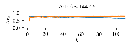
Sortedness over \(k\) per dataset
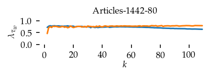
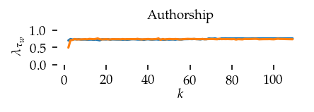
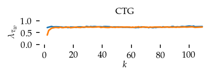
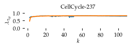
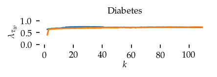
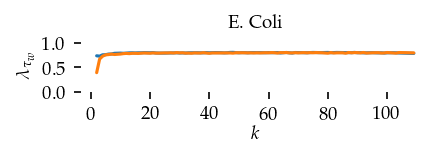
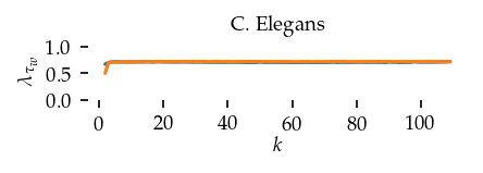
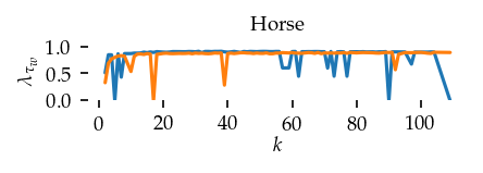
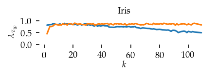
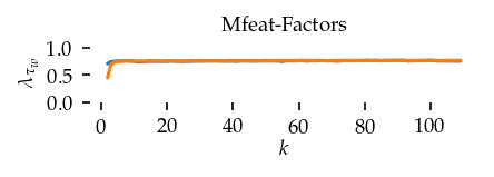
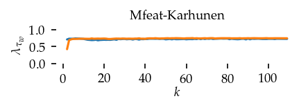
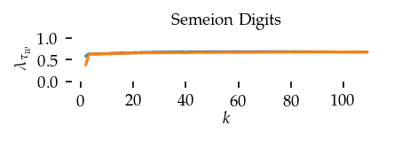
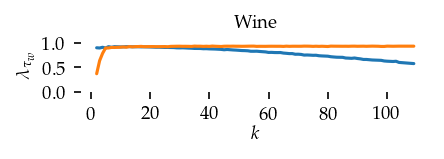
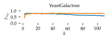
This section draws the average sortedness over k for all datasets. Generally, we see stable performance on both algorithms. The k-NN requires a slightly larger k-value to reach its performance peak. The k-MST performs well on very low k values. On the other hand, its performance drops at higher k-values.
[16]:
for i, data_name in enumerate(datasets):
    sized_fig(0.5, 0.618 / 2)
    ddf = df.query(f'data_set == "{data_name}"')
    max_x = ddf.k.max()
    max_y = ddf.sortedness.max()

    sns.lineplot(
        data=ddf,
        x="k",
        y="sortedness",
        hue="algorithm",
        errorbar=None,
        palette="tab10",
        legend=False,
    )
    plt.title(dataset_name(data_name), fontsize=fontsize['small'])
    plt.ylabel(r"$\lambda_{\tau_w}$")
    plt.xlabel("$k$", labelpad=0)
    plt.ylim(0, 1.05)
    plt.yticks([0, 0.5, 1.0])
    plt.subplots_adjust(bottom=0.38, right=1.01, left=0.16, top=0.78)
    plt.savefig(f"images/sortedness_curves_{data_name}_umap_layout.pdf", pad_inches=0)
plt.show()
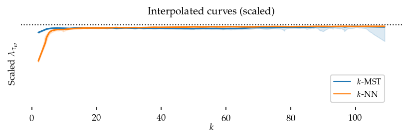
Interpolated curve shape:
To summarize these figures we Lowess interpolate k to the sortedness values considering all datasets. First, we scale the sortedness values by the maximum value observed per dataset so the result captures the curves’ shapes while ignoring absolute performance.
[19]:
def scale_quality(group):
    max_q = group.sortedness.max()
    group["scaled_quality"] = group.sortedness / max_q
    return group


df = df.groupby(["data_set"]).apply(scale_quality, include_groups=False).reset_index()
The resulting figure confirms the previously mentioned patterns: k-MST performs better than k-NN at low k-values (k < 10).
[99]:
sized_fig(1, 0.618 / 2)
max_y = df.scaled_quality.max()
plt.title("Interpolated curves (scaled)")
plt.axhline(y=1, xmin=0, xmax=100, color="k", linestyle=":", linewidth=1)
for j, alg in enumerate(algorithms):
    regplot_lowess_ci(
        df.query(f'algorithm == "{alg}"'),
        x="k",
        y="scaled_quality",
        ci_level=95,
        n_boot=100,
        lowess_frac=0.05,
        color=tab10[j],
        scatter=False,
    )
plt.legend(
    loc="lower right",
    bbox_to_anchor=(0.965, 0),
    handles=[
        plt.Line2D([0], [0], color=tab10[i], lw=1, label=to_display_name(alg))
        for i, alg in enumerate(algorithms)
    ],
)
plt.ylabel(r"Scaled $\lambda_{\tau_w}$")
plt.xlabel("$k$", labelpad=0)
plt.ylim(0, 1.05)
plt.yticks([])
plt.subplots_adjust(bottom=0.2, right=1.02, left=0.09, top=0.88)
plt.savefig(f"images/sortedness_curves_scaled_umap_layout.pdf", pad_inches=0)
plt.show()
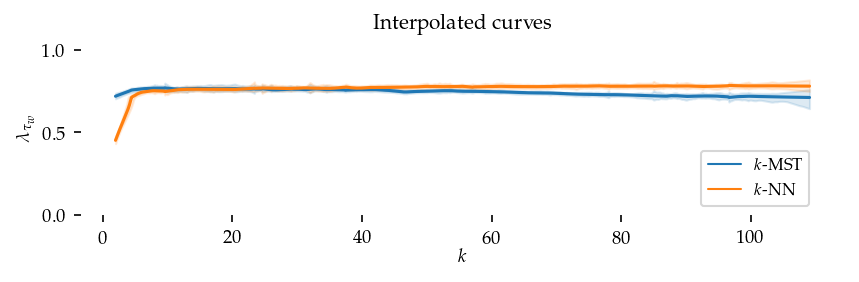
Second, we perform the same interpolation without re-scaling the sortedness. These curves show (local) average sortedness over all datasets. Here, the performance difference at higher k-values (k > 50) is also visible.
[100]:
sized_fig(1, 0.618 / 2)
max_y = df.sortedness.max()
plt.title("Interpolated curves")
for j, alg in enumerate(algorithms):
    regplot_lowess_ci(
        df.query(f'algorithm == "{alg}"'),
        x="k",
        y="sortedness",
        ci_level=95,
        n_boot=100,
        lowess_frac=0.05,
        color=tab10[j],
        scatter=False,
    )
plt.legend(
    loc="lower right",
    bbox_to_anchor=(0.965, 0),
    handles=[
        plt.Line2D([0], [0], color=tab10[i], lw=1, label=to_display_name(alg))
        for i, alg in enumerate(algorithms)
    ],
)
plt.ylabel(r"$\lambda_{\tau_w}$")
plt.xlabel("$k$", labelpad=0)
plt.ylim(0, 1.05)
plt.yticks([0, 0.5, 1.0])
plt.subplots_adjust(bottom=0.2, right=1.02, left=0.09, top=0.88)
plt.savefig(f"images/sortedness_curves_interpolated_umap_layout.pdf", pad_inches=0)
plt.show()
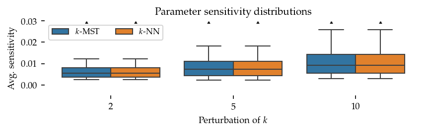
Sensitivity boxplots
The sensitivity analysis computes an average absolute ratio comparing the original and perturbed k values:
where \(V\) is the set of sampled k-values.
This cell computes the sensitivity scores for each dataset.
[ ]:
sensitivity_records = []
for data_set, alg_id in product(datasets, algorithms):
    sub_df = df.query(f"data_set == '{data_set}' & algorithm == '{alg}'")
    vals = defaultdict(
        lambda: np.nan,
        {(r, k): v for r, k, v in zip(sub_df.repeat, sub_df.k, sub_df.sortedness)},
    )
    lookup_fun = np.vectorize(lambda r, x: vals[(r, x)])
    initial_val = np.hstack(
        [lookup_fun(i, min_sample_sizes[:, i])[:, None] for i in range(n_repeats)]
    )
    perturbed_val = np.concatenate(
        [lookup_fun(i, new_values[:, :, i])[:, :, None] for i in range(n_repeats)],
        axis=2,
    )
    with np.errstate(divide="ignore", invalid="ignore"):
        diff = np.abs((perturbed_val - initial_val) / (perturbed_val + initial_val))
    with warnings.catch_warnings():
        warnings.simplefilter("ignore", category=RuntimeWarning)
        sensitivity = np.nanmean(diff, axis=(1, 2))
    for delta, sensitivity in zip(deltas[:, 0], sensitivity):
        sensitivity_records.append(
            {
                "data_set": data_set,
                "alg_id": alg_id,
                "perturbation": delta,
                "sensitivity": sensitivity,
            }
        )

# Convert to pandas
df_sens = pd.DataFrame.from_records(sensitivity_records)
df_sens.head()
| data_set | alg_id | perturbation | sensitivity | |
|---|---|---|---|---|
| 0 | articles_1442_5 | kmst | 2 | 0.006424 |
| 1 | articles_1442_5 | kmst | 5 | 0.007088 |
| 2 | articles_1442_5 | kmst | 10 | 0.011807 |
| 3 | articles_1442_5 | umap | 2 | 0.006424 |
| 4 | articles_1442_5 | umap | 5 | 0.007088 |
There is no visible difference between the sensitivity distributions because the sortedness curves are very flat except at k<10.
[80]:
sized_fig(1, 0.8 / 3)

ax = sns.boxplot(
    data=df_sens,
    y=df_sens.sensitivity,
    x=pd.Categorical(df_sens.perturbation),
    hue=df_sens.alg_id.apply(to_display_name),
    palette=tab10[:2],
    fliersize=0.5,
    linewidth=1,
    legend=True,
)
max_y = 0.03
df_sens.sensitivity > max_y
u_perts = df_sens.perturbation.unique().tolist()
for (alg_id, perturbation), _ in (
    df_sens[df_sens.sensitivity > max_y]
    .groupby(["alg_id", "perturbation"])
    .groups.items()
):
    pert_order = u_perts.index(perturbation)
    alg_order = algorithms.tolist().index(alg_id)
    w = 0.8/2
    o = pert_order - w + (alg_order) * w / 1 + w / 2
    plt.plot(o, max_y - 0.0007, 'k^', markersize=1.5)

# plt.yticks([0, 0.05, 0.1])
plt.ylim(-0.005, max_y)
plt.legend(ncol=4, title="", loc="upper left")
plt.xlabel("Perturbation of $k$")
plt.ylabel("Avg.~sensitivity")
plt.title("Parameter sensitivity distributions")
plt.subplots_adjust(left=0.075, right=1, bottom=0.21, top=0.9)
plt.show()
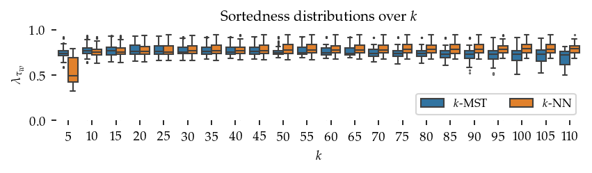
Sortedness distributions
This cell provides an alternative visualization to the interpolated curves. Here, the sortedness is shown in boxplots for segments of k spanning 5 values. The boxplots contain more information than the mean with its confidence interval.
[96]:
sized_fig(1, 0.8 / 3)

ax = sns.boxplot(
    data=df,
    y=df.sortedness,
    x=pd.Categorical(df.k // 5),
    hue=df.algorithm.apply(to_display_name),
    palette=tab10[:2],
    fliersize=0.5,
    linewidth=1,
    legend=True,
)

plt.ylim(-0.005, 1.005)
plt.yticks([0, 0.5, 1])
xticks = plt.xticks()[0]
plt.xticks(xticks)
plt.gca().set_xticklabels([f"{(tick + 1) * 5}" for tick in xticks])
plt.legend(ncol=4, title="", loc="lower right")
plt.xlabel("$k$")
plt.ylabel("$\\lambda_{\\tau_w}$")
plt.title("Sortedness distributions over $k$")
plt.subplots_adjust(left=0.08, right=1, bottom=0.27, top=0.87)
plt.savefig(f"images/sortedness_boxplots_umap_layout.pdf", pad_inches=0)
plt.show()
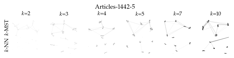
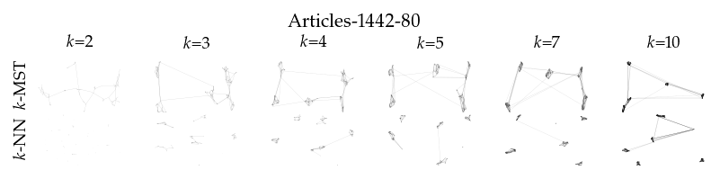
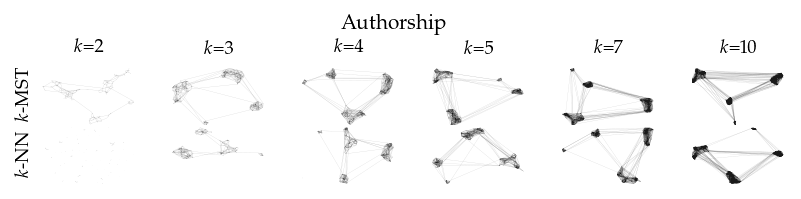
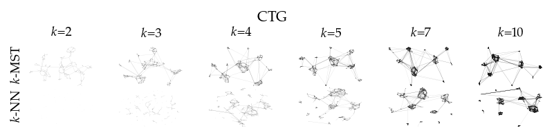
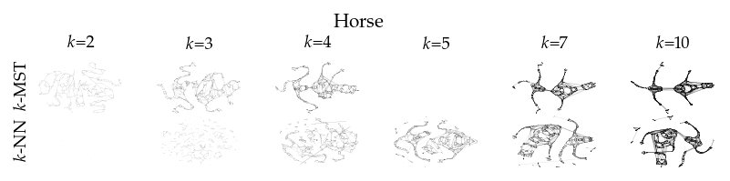
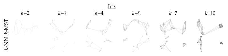
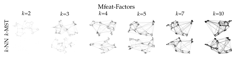
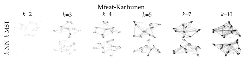
Individual layouts
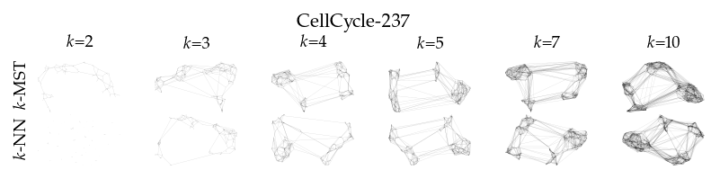
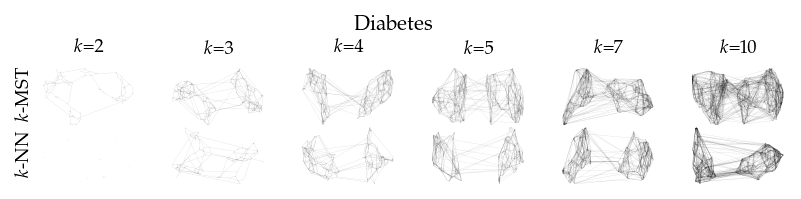
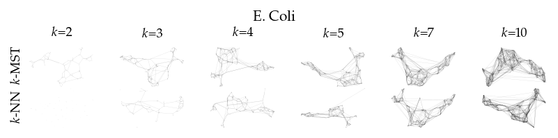
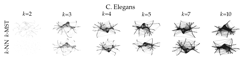
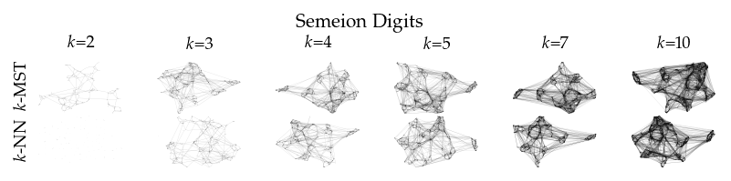
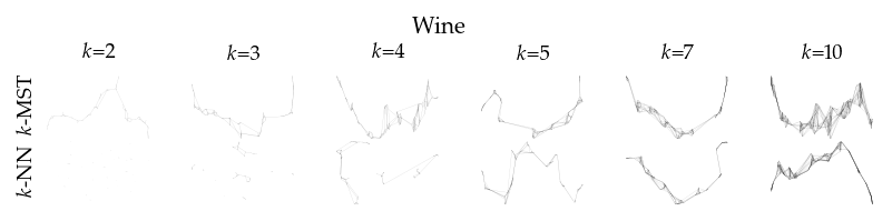
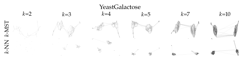
Finally, we draw the edges of the best layout per dataset for select \(k\) values.
[8]:
from sklearn.decomposition import PCA
from matplotlib.collections import LineCollection


plot_ks = [2, 3, 4, 5, 7, 10]
for data_set in datasets:
    sized_fig(1, 0.618 / 6 * 2)
    for i, (alg, k) in enumerate(product(algorithms, plot_ks)):
        plt.subplot(len(algorithms), len(plot_ks), i + 1)
        rows = df.query("data_set == @data_set & k == @k & algorithm == @alg")
        idx = np.argmax(rows.sortedness)
        embedding = rows.embedding.iloc[idx]
        if not np.any(np.isnan(embedding)):
            embedding = PCA().fit_transform(embedding)
        embedding -= embedding.min(axis=0)
        embedding /= embedding.max(axis=0)
        embedding *= np.array([[1.618, 1]])
        graph = rows.graph.iloc[idx].tocoo()
        row, col = graph.row, graph.col
        plt.gca().add_collection(
            LineCollection(
                np.hstack((embedding[row], embedding[col])).reshape(-1, 2, 2),
                alpha=0.1,
                linewidths=0.1,
                color="k",
            )
        )
        plt.xlim(0, 1.668)
        plt.ylim(0, 1.05)
        plt.xticks([])
        plt.yticks([])
        frame_off()
        if alg == algorithms[0]:
            plt.title(f"$k$={k}", fontsize=fontsize["small"])
        if k == plot_ks[0]:
            plt.ylabel(to_display_name(alg), fontsize=fontsize["small"])
        plt.suptitle(dataset_name(data_set), fontsize=fontsize["normal"], y=1, va="top")
    plt.subplots_adjust(0.05, 0, 1, 0.7, 0, 0)
    plt.savefig(f"images/umap_layouts_{data_set}.png", pad_inches=0)
plt.show()