Changing the data | Data Visualisation in Data Science

If your dataset is a bit bigger than what you see here, it’ll become impossible to type this into the specification. It’s often better to load your data from an external source. Looking at the documentation we see that data can be inline, or loaded from a URL. There is also something called “Named data sources”, but we won’t look into that here.

Accessing public data

What we’ve done above is provide the data inline. In that case, you need the values key, e.g.

"data": {
  "values": [
    {"a": "A", "b": 28},
    {"a": "B", "b": 55}
  ]
}

When loading external data, we’ll need the url key instead:

"data": {
  "url": "https://raw.githubusercontent.com/vega/vega/master/docs/data/cars.json"
}

This cars dataset is one of the standard datasets used for learning data visualisation. The json file at the URL looks like this:

[
   {
      "Name":"chevrolet chevelle malibu",
      "Miles_per_Gallon":18,
      "Cylinders":8,
      "Displacement":307,
      "Horsepower":130,
      "Weight_in_lbs":3504,
      "Acceleration":12,
      "Year":"1970-01-01",
      "Origin":"USA"
   },
   {
      "Name":"buick skylark 320",
      "Miles_per_Gallon":15,
      "Cylinders":8,
      "Displacement":350,
      ...}
]

So it is an array ([]) of objects ({}) where each object is a car for which we have a name, miles per gallon, cylinders, etc.

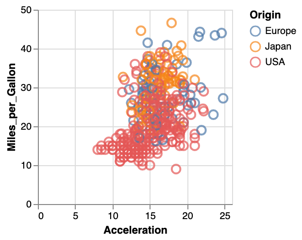
Exercise 5: Alter the specification in the vega-lite editor to recreate this image:

How to use your own data

Using a public online dataset like the one above is simple. But how can you access your own data? What if you have an Excel file with data that you want to visualise?

Gist

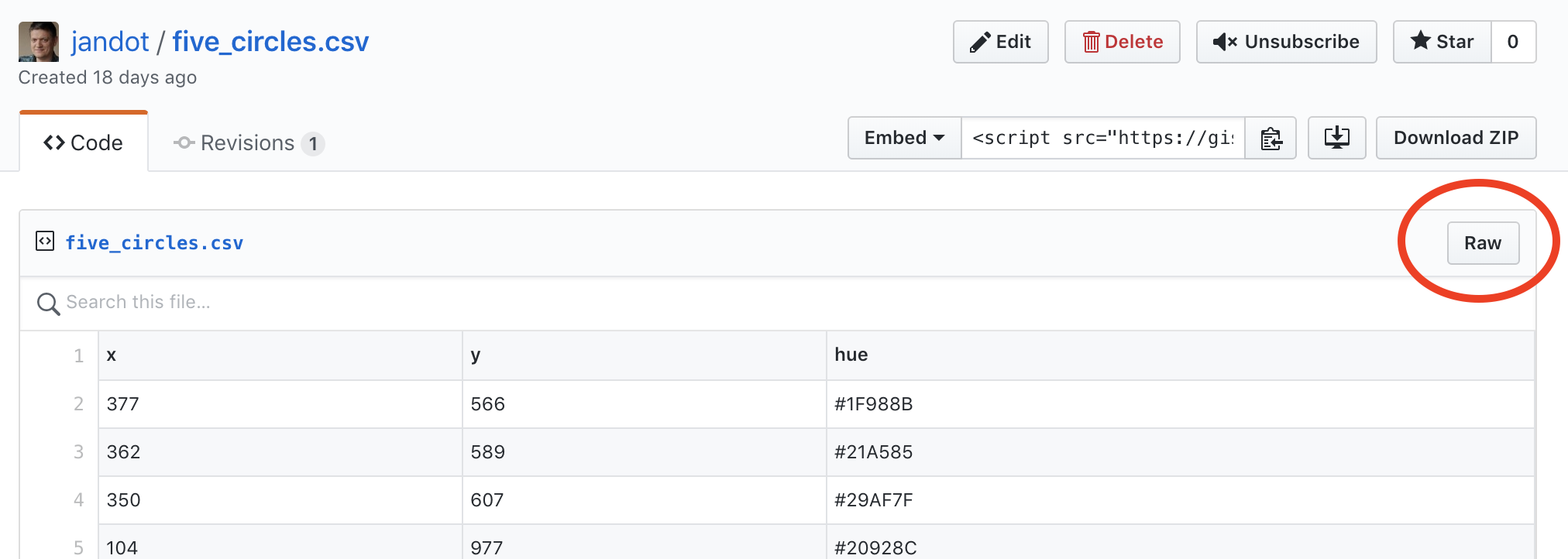
If your data is not sensitive, you can use github “gists” at https://gist.github.com/. This provides you with a space where you can upload your csv or json data and will return a URL that you can use as we did above.

The URL to use should be the one that you see after you clicked the button named “Raw” in the top-right. This will be the actual data.

For example:

Here is information how to create new gists.

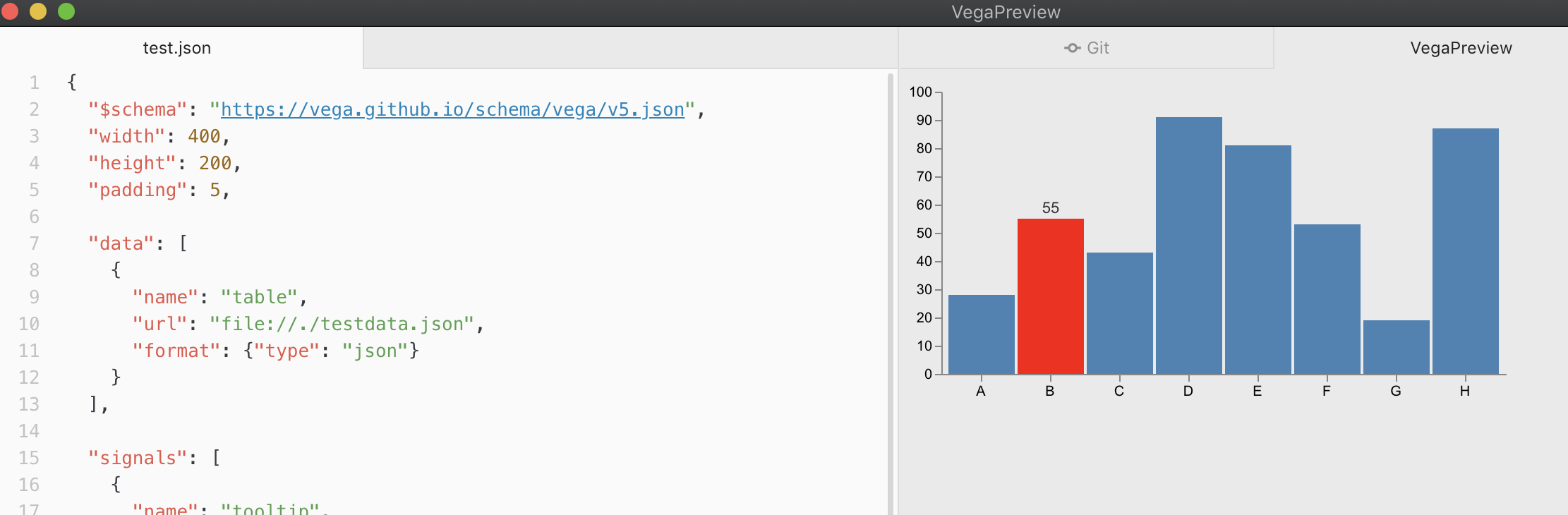
In an IDE

Another option is to use an IDE (integrated development environment) or code editor which can interpret vega specifications. The atom editor, for example, has a vega-preview package. In this case, you don’t have to upload your data to an external website. Instead, you can use file:// as part of the url instead of http://

Local server

Finally, you can also run a local webserver where you can load an html-file with embedded vega code. You might be able to run a local server by running python -m SimpleHTTPServer, or install http-server from https://www.npmjs.com/package/http-server.

With this server running, create an html file that looks like this:

<head>
  <script src="https://cdn.jsdelivr.net/npm/vega@5"></script>
  <script src="https://cdn.jsdelivr.net/npm/vega-lite@4"></script>
  <script src="https://cdn.jsdelivr.net/npm/vega-embed@6"></script>
</head>
<body>
  <div id="vis1"></div>
  <script type="text/javascript">
    var yourVlSpec = {
      "$schema": "https://vega.github.io/schema/vega-lite/v4.json",
      "title": "Side-by-side plots",
      "data": {
        "url": "https://raw.githubusercontent.com/vega/vega/master/docs/data/cars.json"
      },
      "transform": [
        { "calculate": "year(datum.Year)", "as": "yearonly" }

      ],
      "concat": [
        {
          "mark": "circle",
          "encoding": {
            "x": {"field": "Acceleration", "type": "quantitative"},
            "y": {"field": "Miles_per_Gallon", "type": "quantitative"},
            "color": {"field": "yearonly", "type": "ordinal"}
          }
        },
        {
          "mark": "circle",
          "encoding": {
            "x": {"field": "Horsepower", "type": "quantitative"},
            "y": {"field": "Miles_per_Gallon", "type": "quantitative"},
            "color": {"field": "yearonly", "type": "ordinal"}
          }
        }
      ]
    };
    vegaEmbed('#vis1', yourVlSpec);
</body>

Note that you create a div named vis1 into which you will embed the yourVlSpec specification. (Note: this is actually how all interactive vega-lite and vega visualisations in this tutorial are embedded in the website.)

Exercise - Copy the data below into a local file, and visualise it however you want (scatterplot, barchart, 3D pie chart, …) without copy/pasting it directly in the specification. In other words: the specification should use url for the data, not values.

CRIM,ZN,INDUS,CHAS,NOX,RM,AGE,DIS,RAD,TAX,PTRATIO,B,LSTAT,MEDV
0.00632,18.00,2.310,0,0.5380,6.5750,65.20,4.0900,1,296.0,15.30,396.90,4.98,24.00
0.02731,0.00,7.070,0,0.4690,6.4210,78.90,4.9671,2,242.0,17.80,396.90,9.14,21.60
0.02729,0.00,7.070,0,0.4690,7.1850,61.10,4.9671,2,242.0,17.80,392.83,4.03,34.70
0.03237,0.00,2.180,0,0.4580,6.9980,45.80,6.0622,3,222.0,18.70,394.63,2.94,33.40
0.06905,0.00,2.180,0,0.4580,7.1470,54.20,6.0622,3,222.0,18.70,396.90,5.33,36.20
0.02985,0.00,2.180,0,0.4580,6.4300,58.70,6.0622,3,222.0,18.70,394.12,5.21,28.70
0.08829,12.50,7.870,0,0.5240,6.0120,66.60,5.5605,5,311.0,15.20,395.60,12.43,22.90
0.14455,12.50,7.870,0,0.5240,6.1720,96.10,5.9505,5,311.0,15.20,396.90,19.15,27.10
0.21124,12.50,7.870,0,0.5240,5.6310,100.00,6.0821,5,311.0,15.20,386.63,29.93,16.50
0.17004,12.50,7.870,0,0.5240,6.0040,85.90,6.5921,5,311.0,15.20,386.71,17.10,18.90

Explanation of the column names:
CRIM: per capita crime rate by town
ZN: proportion of residential land zoned for lots over 25,000 sq.ft.
INDUS: proportion of non-retail business acres per town
CHAS: Charles River dummy variable (= 1 if tract bounds river; 0 otherwise)
NOX: nitric oxides concentration (parts per 10 million)
RM: average number of rooms per dwelling
AGE: proportion of owner-occupied units built prior to 1940
DIS: weighted distances to five Boston employment centres
RAD: index of accessibility to radial highways
TAX: full-value property-tax rate per $10,000
PTRATIO: pupil-teacher ratio by town
B: 1000(Bk - 0.63)^2 where Bk is the proportion of blacks by town
LSTAT: % lower status of the population
MEDV: Median value of owner-occupied homes in $1000’s